Minocycline (Athanassa 2025)
Source:vignettes/articles/Athanassa_2025_minocycline.Rmd
Athanassa_2025_minocycline.RmdModel and source
- Citation: Athanassa Z, Papakyriakopoulou P, Marquez Megias S, Saitani EM, Manioudaki S, Dimoula K, Petsa I, Valsami G, Sakagianni A, Koumaki V, Dokoumetzidis A, Tsakris A. Population pharmacokinetic model of oral minocycline in critically ill adult patients with ventilator-associated pneumonia. J Antimicrob Chemother. 2025;80(5):1420-1426. doi:10.1093/jac/dkaf090.
- Description: One-compartment population PK model with first-order absorption and linear elimination for orally administered minocycline in critically ill adults with ventilator-associated pneumonia caused by multidrug-resistant Acinetobacter baumannii (Athanassa 2025). Minocycline was given by mouth (dispersed in water, via nasogastric or orogastric tube in mechanically ventilated patients) as a 200 mg loading dose followed by 100 mg every 12 h. The model is parameterized in apparent oral terms: apparent clearance CL/F 6.55 L/h, apparent central volume V/F 183.3 L, and absorption rate constant ka 1.66 1/h, which together imply a terminal half-life of 19.4 h and an absorption half-life of 0.42 h (25 min), both as quoted in the paper’s Discussion. Between-subject variability is exponential on CL/F (omega 0.59 on the log scale) and V/F (omega 1.16); variability on ka was tested but was not estimable from these data and is absent from the final model. Residual error is proportional (0.616). Nine covariates (age, sex, body weight, BMI, serum albumin, creatinine, creatinine clearance, haematocrit and SOFA score) were screened; none was retained, so the final model is covariate-free (see covariatesDataExcluded).
- Article: J Antimicrob Chemother 2025;80(5):1420-1426
Athanassa and colleagues ran a prospective, open-label study of orally administered minocycline in critically ill ICU adults with ventilator-associated pneumonia (VAP) caused by multidrug-resistant Acinetobacter baumannii. Almost all published minocycline PK comes from 1970s intravenous studies using bioassay methods, so this is one of very few modern population models for the oral route, and the only one in a critically ill population.
The final model is deliberately simple: one compartment, first-order absorption, linear elimination, exponential between-subject variability on CL/F and V/F, proportional residual error, and no covariates.
Population
The model was built from 24 critically ill adults (17 male, 7 female) treated in the ICU of Sismanogleio General Hospital, Athens, between August 2021 and April 2023. Median age was 69.5 years (IQR 63-76.5) and median weight 85.0 kg (IQR 70.0-106.5). All were mechanically ventilated with microbiologically confirmed A. baumannii VAP, diagnosed after a median ICU stay of 16 days; 84% had been admitted for COVID-19. The cohort was severely ill (median SOFA score 9, IQR 8-10) and markedly hypoalbuminaemic (median serum albumin 2.45 g/dL). Renal function was impaired in many: measured creatinine clearance (24-h urine collection) had a median of 57.7 mL/min (IQR 28.5-104), with 11 of 24 patients below 50 mL/min and none on renal replacement therapy. Baseline characteristics are from Athanassa 2025 Table 1.
Every patient received minocycline dispersed in water as a 200 mg loading dose followed by 100 mg every 12 h for at least 5 days; mechanically ventilated patients received it through a nasogastric or orogastric tube. Of 182 plasma concentrations collected, 10 (5.49%) were below the limit of quantification and discarded, leaving 172 for model development. Sampling was sparse and schedule-dependent: 20 patients were sampled at 12, 13, 14, 18, 21.5, 48, 59.5, 61, 64, 68 and 71.5 h, and 4 patients at 0.5, 1, 2, 4, 6 and 12 h. That sampling design matters for the validation below, because the paper’s reported Tmax values are quantised onto this grid.
The same information is available programmatically via the model’s
population metadata
(readModelDb("Athanassa_2025_minocycline")()$population).
pop <- rxode2::rxode(readModelDb("Athanassa_2025_minocycline"))$population
#> ℹ parameter labels from comments will be replaced by 'label()'
tibble::tibble(Field = names(pop), Value = vapply(pop, paste, character(1), collapse = "; ")) |>
knitr::kable(caption = "Study population metadata carried in the model file.")| Field | Value |
|---|---|
| species | human |
| n_subjects | 24 |
| n_studies | 1 |
| n_observations | 172 |
| age_median | 69.5 years (IQR 63-76.5) |
| weight_median | 85.0 kg (IQR 70.0-106.5) |
| bmi_median | 25 kg/m^2 (IQR 23.95-32.5) |
| sex_female_pct | 29.2 |
| disease_state | Critically ill mechanically-ventilated ICU adults with ventilator-associated pneumonia caused by multidrug-resistant Acinetobacter baumannii; median SOFA score 9 (IQR 8-10) at admission; 84% admitted for COVID-19 infection; VAP diagnosed after a median ICU stay of 16 days |
| renal_function | Measured creatinine clearance (24-h urine collection) median 57.7 mL/min (IQR 28.5-104); 11 of 24 patients had CLCR < 50 mL/min, none on renal replacement therapy |
| dose_range | 200 mg oral loading dose, then 100 mg every 12 h for at least 5 days |
| co_medication | Colistin 67%, meropenem 29%, ampicillin-sulbactam 29% |
| regions | Greece (single centre: Sismanogleio General Hospital, Athens; August 2021 to April 2023) |
| notes | Baseline demographics from Athanassa 2025 Table 1. 182 plasma minocycline concentrations were collected; 10 (5.49%) below the limit of quantification were discarded, leaving 172 used for model development. Sampling was sparse: 20 patients were sampled at 12, 13, 14, 18, 21.5, 48, 59.5, 61, 64, 68 and 71.5 h and 4 patients at 0.5, 1, 2, 4, 6 and 12 h. Minocycline MICs were 4 mg/L or lower in 13 strains (susceptible) and 8 mg/L in 11 strains (intermediate). Serum albumin was low throughout (median 2.45 g/dL), which the authors cite as the reason the albumin-on-volume effect was poorly identified. |
Source trace
The per-parameter origin is recorded as an in-file comment next to
each ini() entry in
inst/modeldb/specificDrugs/Athanassa_2025_minocycline.R.
The table below collects them in one place for review.
| Equation / parameter | Value | Source location |
|---|---|---|
lka (ka) |
1.66 1/h | Table 2, “Ka (1/h)”, Final model Estimate (41.9% RSE); restated in the Abstract |
lcl (CL/F) |
6.55 L/h | Table 2, “CL/F (L/h)”, Final model Estimate (17.2% RSE); restated in the Abstract |
lvc (V/F) |
183.3 L | Table 2, “V/F (L)”, Final model Estimate (25.9% RSE); restated in the Abstract |
etalcl |
omega 0.59 (variance 0.3481) | Table 2, “IIV-CL/F”, Final model Estimate (23.8% RSE), %CV 64%, shrinkage 16.9% |
etalvc |
omega 1.16 (variance 1.3456) | Table 2, “IIV-V/F”, Final model Estimate (16.4% RSE), shrinkage -2.7% |
propSd |
0.616 | Table 2, “Proportional error”, Final model Estimate (5.9% RSE) |
| One compartment, first-order absorption, linear elimination | n/a | Abstract; Results, “popPK model” |
| No lag time | n/a | Methods, “Population PK model development” (Tlag tested, not retained) |
| No IIV on ka | n/a | Results, “popPK model”: IIV “could not be estimated on ka” |
| No covariates | n/a | Results, “Covariate analysis” (see
covariatesDataExcluded in the model file) |
| Apparent (oral) parameterisation, no explicit F | n/a | Results, “popPK model”: parameterised as CL/F and V/F |
| Protein binding 76% (fu = 0.24), used only for PTA | n/a | Methods, “PTA simulations”; Discussion |
Two derived quantities quoted in the paper’s Discussion act as independent arithmetic checks on the structural parameters, and are asserted in the next section:
- terminal half-life
log(2) * (V/F) / (CL/F)= 19.4 h (“the model’s estimated average t 1/2 of 19.4 h”); - absorption half-life
log(2) / ka= 0.42 h, i.e. 25 min (“an absorption t 1/2 of 0.42 h (25 min)”).
Structural checks
These are deterministic identities of the packaged model, evaluated on the typical-value profile with between-subject variability zeroed. Each is asserted, so this vignette fails to build if a future edit perturbs the structure.
mod     <- readModelDb("Athanassa_2025_minocycline")
mod_typ <- rxode2::zeroRe(mod)
#> ℹ parameter labels from comments will be replaced by 'label()'

# Regimen actually studied: 200 mg oral loading dose, then 100 mg q12h.
dose_times <- c(0, seq(12, 60, by = 12))
ev_typ <-
  rxode2::et(amt = 200, time = 0, cmt = "depot") |>
  rxode2::et(amt = 100, time = 12, cmt = "depot", ii = 12, addl = 4) |>
  rxode2::et(seq(0, 156, by = 0.05), cmt = "central")

sim_typ <- rxode2::rxSolve(mod_typ, ev_typ, returnType = "data.frame")
#> ℹ omega/sigma items treated as zero: 'etalcl', 'etalvc'

# 1. Terminal half-life, recovered from the log-linear slope well after the
#    final dose (>= 24 h post-dose, so the absorption transient has decayed).
tail_fit  <- lm(log(Cc) ~ time, data = subset(sim_typ, time >= 84 & time <= 156))
thalf_sim <- log(2) / -coef(tail_fit)[["time"]]
thalf_an  <- log(2) * 183.3 / 6.55

# 2. Absorption half-life.
thalf_abs <- log(2) / 1.66

# 3. Steady-state exposure identity: AUC over a dosing interval at steady
#    state equals Dose / CL, independent of volume.
auc_ss_an <- 100 / 6.55

tibble::tibble(
  Check = c(
    "Terminal half-life (analytic, log(2)*V/CL)",
    "Terminal half-life (simulated terminal slope)",
    "Absorption half-life (log(2)/ka)",
    "AUC0-tau at steady state (Dose/CL, 100 mg q12h)"
  ),
  Model     = c(thalf_an, thalf_sim, thalf_abs, auc_ss_an),
  Published = c(19.4, 19.4, 0.42, NA_real_),
  Units     = c("h", "h", "h", "mg*h/L")
) |>
  knitr::kable(digits = 3,
caption = "Structural identities versus the values quoted in the Athanassa 2025 Discussion.")| Check | Model | Published | Units |
|---|---|---|---|
| Terminal half-life (analytic, log(2)*V/CL) | 19.398 | 19.40 | h |
| Terminal half-life (simulated terminal slope) | 19.398 | 19.40 | h |
| Absorption half-life (log(2)/ka) | 0.418 | 0.42 | h |
| AUC0-tau at steady state (Dose/CL, 100 mg q12h) | 15.267 | NA | mg*h/L |
# Assertions -- these make the vignette fail loudly on a structural regression.
stopifnot(
  abs(thalf_an  - 19.4) < 0.05,
  abs(thalf_sim - 19.4) < 0.05,
  abs(thalf_abs - 0.42) < 0.005
)
Both published derived quantities are reproduced to the precision at which the paper states them, which confirms that CL/F, V/F and ka were transcribed on the correct scale.
Virtual cohort
Original observed data are not publicly available. The cohort below is a virtual population of 200 subjects per sampling arm, dosed on the studied regimen. The model carries no covariates, so no covariate distribution has to be assumed – between-subject variability enters entirely through the two etas.
Two arms mirror the study’s two sampling schedules (Athanassa 2025 Methods), so that the observation process, not just the underlying profile, is replicated:
- sparse – the 20-patient schedule (12, 13, 14, 18, 21.5, 48, 59.5, 61, 64, 68, 71.5 h);
- rich – the 4-patient early schedule (0.5, 1, 2, 4, 6, 12 h).
A third dense arm on a fine grid supports the VPC and the NCA below.
set.seed(20250326)
n_per_arm <- 200

# Dose rows are written out one per administration rather than with `addl`,
# so that the dose frame handed to PKNCA below carries all six doses.
make_cohort <- function(n, times, arm, id_offset = 0L) {
  base <-
    rxode2::et(amt = c(200, rep(100, 5)), time = dose_times, cmt = "depot") |>
    rxode2::et(times, cmt = "central") |>
    as.data.frame()
  do.call(rbind, lapply(seq_len(n), function(i) {
    transform(base, id = id_offset + i, arm = arm)
  }))
}

events <- dplyr::bind_rows(
  make_cohort(n_per_arm, c(0, 0.5, 1, 2, 4, 6, 12), "rich", id_offset = 0L),
  make_cohort(n_per_arm, c(0, 12, 13, 14, 18, 21.5, 48, 59.5, 60, 61, 64, 68, 71.5),
              "sparse", id_offset = 1000L),
  make_cohort(n_per_arm, seq(0, 84, by = 0.25), "dense", id_offset = 2000L)
)

stopifnot(!anyDuplicated(events[, c("id", "time", "evid")]))
Simulation
Cc is the individual prediction (IPRED);
sim additionally carries the proportional residual error
and is the simulated observation. Both are used below, for
different purposes: structural and NCA comparisons use Cc,
while the VPC and the observation-process check use
sim.
sim <- rxode2::rxSolve(mod, events = events, keep = "arm", returnType = "data.frame")
#> ℹ parameter labels from comments will be replaced by 'label()'

# The paper discarded concentrations below the limit of quantification
# (10 of 182, 5.49%). Its reported concentration range bottoms out at
# 0.06 mg/L (Table 1), which is used here as the LOQ. This also removes the
# negative draws that a 61.6% proportional error model inevitably produces.
LOQ <- 0.06
sim <- sim |>
  dplyr::mutate(
    obs = dplyr::if_else(sim >= LOQ, sim, NA_real_),
    tad = time - dose_times[findInterval(time, dose_times)]
  )

sprintf("Simulated BLQ fraction: %.1f%% (paper discarded 5.49%%)",
        100 * mean(is.na(sim$obs[sim$time > 0])))
#> [1] "Simulated BLQ fraction: 8.8% (paper discarded 5.49%)"
Replicate published figures
Figure 1 – visual predictive check
The paper presents the VPC “with respect to the time after dose”, with the 5th, 50th and 95th percentiles of observations. The panel below reproduces that presentation from the packaged model.
# Replicates Figure 1 of Athanassa 2025: VPC of concentration vs. time after dose.
sim |>
  dplyr::filter(arm == "dense", time > 0, !is.na(obs)) |>
  dplyr::mutate(tad_bin = round(tad * 2) / 2) |>
  dplyr::group_by(tad_bin) |>
  dplyr::summarise(
    Q05 = quantile(obs, 0.05),
    Q50 = quantile(obs, 0.50),
    Q95 = quantile(obs, 0.95),
    .groups = "drop"
  ) |>
  ggplot(aes(tad_bin, Q50)) +
  geom_ribbon(aes(ymin = Q05, ymax = Q95), alpha = 0.25) +
  geom_line(linewidth = 0.8) +
  scale_y_log10() +
  labs(
    x = "Time after dose (h)", y = "Minocycline concentration (mg/L)",
    title = "Figure 1 - VPC of simulated observations by time after dose",
    caption = "Replicates Figure 1 of Athanassa 2025."
  ) +
  theme_bw()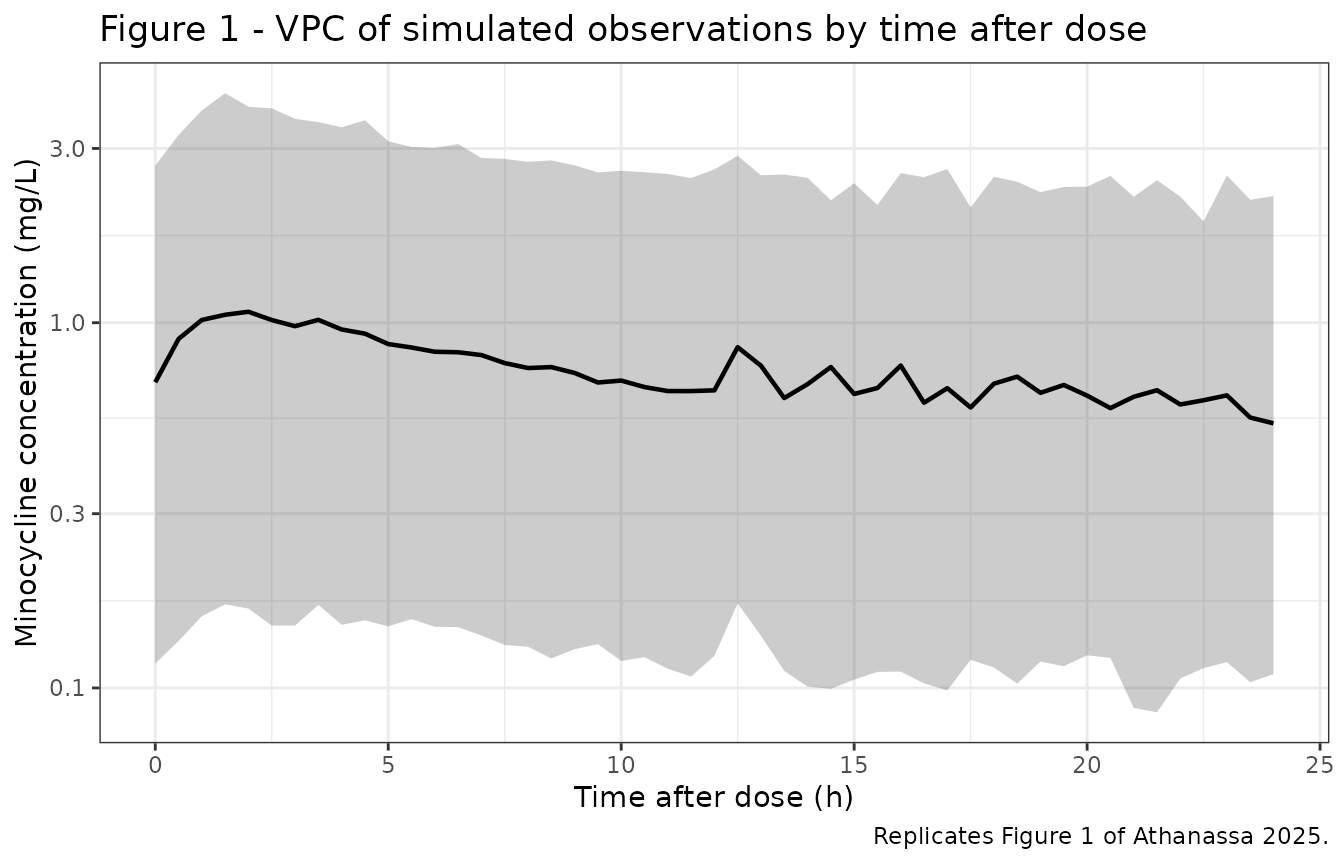
The wide band during the first few hours reproduces the paper’s own observation that “greater variability is observed during the absorption phase and initial distribution of the drug at earlier time points, resulting in wider CI.”
Figure 2 – probability of target attainment
The PTA analysis is a clean, independent check on CL/F and its variability, because at steady state AUC = Dose/CL exactly – the volume and ka drop out. Following the paper’s Methods, 10 000 AUC values are generated for a 400 mg daily dose, converted to free AUC assuming 76% protein binding (fu = 0.24), and divided by a range of MICs.
set.seed(20250326)
n_mc      <- 10000
daily_dose <- 400   # mg/day, the maximum daily dose in the MINOCIN SPC
fu         <- 0.24  # 76% protein binding

cl_mc  <- 6.55 * exp(rnorm(n_mc, 0, 0.59))     # lognormal CL/F, omega = 0.59
fauc_mc <- fu * daily_dose / cl_mc             # free AUC0-24 at steady state

mics    <- c(0.062, 0.125, 0.25, 0.5, 1, 2, 4)
targets <- c(13.75, 25)

pta <- tidyr::expand_grid(MIC = mics, target = targets) |>
  dplyr::rowwise() |>
  dplyr::mutate(PTA = 100 * mean(fauc_mc / MIC > target)) |>
  dplyr::ungroup() |>
  dplyr::mutate(target = factor(target, levels = targets,
                                labels = c("fAUC/MIC > 13.75", "fAUC/MIC > 25")))

ggplot(pta, aes(MIC, PTA, colour = target, shape = target)) +
  geom_line(linewidth = 0.8) + geom_point(size = 2) +
  geom_hline(yintercept = 90, linetype = "dashed") +
  scale_x_log10(breaks = mics) +
  labs(
    x = "MIC (mg/L)", y = "PTA (%)", colour = NULL, shape = NULL,
    title = "Figure 2 - PTA for 400 mg daily minocycline",
    caption = "Replicates Figure 2 of Athanassa 2025. Dashed line = 90% PTA."
  ) +
  theme_bw() + theme(legend.position = "bottom")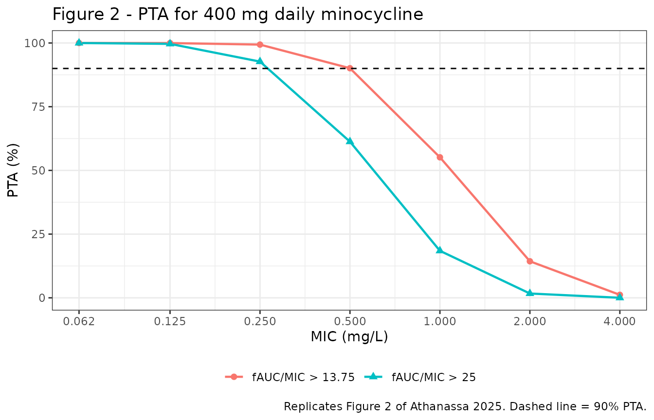
pta |>
  dplyr::mutate(PTA = sprintf("%.1f", PTA)) |>
  tidyr::pivot_wider(names_from = target, values_from = PTA) |>
  dplyr::mutate(MIC = format(MIC, trim = TRUE, drop0trailing = TRUE)) |>
  dplyr::rename("MIC (mg/L)" = MIC) |>
knitr::kable(caption = "PTA (%) by MIC for a 400 mg daily dose.")| MIC (mg/L) | fAUC/MIC > 13.75 | fAUC/MIC > 25 |
|---|---|---|
| 0.062 | 100.0 | 100.0 |
| 0.125 | 100.0 | 99.7 |
| 0.25 | 99.4 | 92.7 |
| 0.5 | 90.1 | 61.3 |
| 1 | 55.1 | 18.4 |
| 2 | 14.3 | 1.7 |
| 4 | 1.2 | 0.0 |
This reproduces both breakpoints the paper reports. For the stringent
fAUC/MIC > 25 target, PTA is high at MIC 0.25 mg/L and then falls
away sharply – the paper states that PTA “drops rapidly for MIC >
0.25 mg/L”. For the more permissive fAUC/MIC > 13.75 target, high PTA
is “maintained up to MIC = 0.5 mg/L, beyond which PTA declines rapidly”.
The typical-value arithmetic behind the curves is
fAUC = 0.24 * 400 / 6.55 = 14.66 mg*h/L, so the typical
fAUC/MIC is 58.6 at MIC 0.25, 29.3 at MIC 0.5 and 14.7 at MIC 1.
PKNCA validation
NCA is computed with PKNCA on the dense arm, over two dosing intervals: the second dose (12-24 h, the first 100 mg maintenance dose) and the sixth dose (60-72 h), both of which the paper reports on.
sim_nca <- sim |>
  dplyr::filter(arm == "dense", !is.na(Cc)) |>
  dplyr::mutate(
    treatment = "200 mg load + 100 mg q12h"
  ) |>
  dplyr::select(id, time, Cc, treatment)

# Guarantee a time = 0 record per subject; pre-dose Cc = 0 for an
# extravascular model. Existing time = 0 rows win.
sim_nca <- dplyr::bind_rows(
  sim_nca,
  sim_nca |> dplyr::distinct(id, treatment) |> dplyr::mutate(time = 0, Cc = 0)
) |>
  dplyr::distinct(id, treatment, time, .keep_all = TRUE) |>
  dplyr::arrange(id, treatment, time)

dose_df <- events |>
  dplyr::filter(arm == "dense", evid != 0) |>
  dplyr::mutate(treatment = "200 mg load + 100 mg q12h") |>
  dplyr::select(id, time, amt, treatment)

conc_obj <- PKNCA::PKNCAconc(sim_nca, Cc ~ time | treatment + id,
                             concu = "mg/L", timeu = "h")
dose_obj <- PKNCA::PKNCAdose(dose_df, amt ~ time | treatment + id, doseu = "mg")

intervals <- data.frame(
  start   = c(12, 60),
  end     = c(24, 72),
  cmax    = TRUE,
  tmax    = TRUE,
  cmin    = TRUE,
  cav     = TRUE,
  auclast = TRUE
)

nca_res <- PKNCA::pk.nca(PKNCA::PKNCAdata(conc_obj, dose_obj, intervals = intervals))

nca_tbl <- as.data.frame(nca_res$result) |>
  dplyr::mutate(dose_no = dplyr::if_else(start == 12, "Dose 2 (12-24 h)", "Dose 6 (60-72 h)")) |>
  dplyr::group_by(dose_no, PPTESTCD) |>
  dplyr::summarise(
    Median = median(PPORRES, na.rm = TRUE),
    Mean   = mean(PPORRES, na.rm = TRUE),
    P05    = quantile(PPORRES, 0.05, na.rm = TRUE),
    P95    = quantile(PPORRES, 0.95, na.rm = TRUE),
    .groups = "drop"
  ) |>
  dplyr::mutate(Parameter = nlmixr2lib::ncaParamLabel(as.character(PPTESTCD))) |>
  dplyr::select(dose_no, Parameter, Median, Mean, P05, P95)

nca_tbl |>
  dplyr::rename("Dosing interval" = dose_no) |>
  knitr::kable(digits = 3,
caption = "Simulated NCA (n = 200, individual predictions) over two dosing intervals.")| Dosing interval | Parameter | Median | Mean | P05 | P95 |
|---|---|---|---|---|---|
| Dose 2 (12-24 h) | AUClast | 9.355 | 11.104 | 2.332 | 26.461 |
| Dose 2 (12-24 h) | Cavg | 0.780 | 0.925 | 0.194 | 2.205 |
| Dose 2 (12-24 h) | Cmax | 0.991 | 1.223 | 0.199 | 2.808 |
| Dose 2 (12-24 h) | Cmin | 0.478 | 0.579 | 0.088 | 1.426 |
| Dose 2 (12-24 h) | Tmax | 2.000 | 2.018 | 1.250 | 3.000 |
| Dose 6 (60-72 h) | AUClast | 12.073 | 13.870 | 4.454 | 28.931 |
| Dose 6 (60-72 h) | Cavg | 1.006 | 1.156 | 0.371 | 2.411 |
| Dose 6 (60-72 h) | Cmax | 1.297 | 1.456 | 0.418 | 3.025 |
| Dose 6 (60-72 h) | Cmin | 0.719 | 0.850 | 0.113 | 1.845 |
| Dose 6 (60-72 h) | Tmax | 1.750 | 1.849 | 1.250 | 2.500 |
The accumulation between the second and sixth dose is modest but real, as expected for a 19.4 h half-life on a 12 h dosing interval.
Comparison against published values
The paper reports observed Cmax and Tmax in its Discussion rather than a formal NCA table: “A second 100 mg oral dose at 12 h resulted in a Cmax of 1.23 mg/L, and after the sixth dose, mean Cmax values ranged from 1.9 to 2.04 mg/L”, and “Our Tmax observations of 2 h after the first and second doses, and 1 h after the sixth dose”. The dose-6 Cmax reference below is the midpoint of the reported 1.9-2.04 mg/L range.
The model side of the comparison is the typical-value prediction (between- subject variability zeroed, fine time grid). That choice is deliberate: with omega values of 0.59 and 1.16 the simulated Cmax distribution is extremely heavy-tailed, so a 200-subject cohort median or mean carries visible Monte Carlo noise, whereas the typical-value prediction is a deterministic property of the packaged model and is reproducible exactly.
# Typical-value profile on a fine grid so Tmax is resolved, not snapped to the
# cohort's 0.25 h grid. rxSolve omits `id` for a single subject, so add it.
sim_typ_nca <- rxode2::rxSolve(
  mod_typ,
  rxode2::et(amt = c(200, rep(100, 5)), time = dose_times, cmt = "depot") |>
    rxode2::et(seq(0, 84, by = 0.02), cmt = "central"),
  returnType = "data.frame"
) |>
  dplyr::mutate(id = 1L, treatment = "typical") |>
  dplyr::filter(!is.na(Cc)) |>
  dplyr::select(id, time, Cc, treatment)
#> ℹ omega/sigma items treated as zero: 'etalcl', 'etalvc'

dose_typ <- data.frame(id = 1L, time = dose_times,
                       amt = c(200, rep(100, 5)), treatment = "typical")

nca_typ <- PKNCA::pk.nca(PKNCA::PKNCAdata(
  PKNCA::PKNCAconc(sim_typ_nca, Cc ~ time | treatment + id,
                   concu = "mg/L", timeu = "h"),
  PKNCA::PKNCAdose(dose_typ, amt ~ time | treatment + id, doseu = "mg"),
  intervals = data.frame(start = c(12, 60), end = c(24, 72),
                         cmax = TRUE, tmax = TRUE)
))

published <- tibble::tribble(
  ~dose_no,             ~cmax, ~tmax,
  "Dose 2 (12-24 h)",   1.23,  2,
  "Dose 6 (60-72 h)",   1.97,  1
)

cmp <- nlmixr2lib::ncaComparisonTable(
  simulated     = as.data.frame(nca_typ$result) |>
    dplyr::mutate(dose_no = dplyr::if_else(start == 12, "Dose 2 (12-24 h)", "Dose 6 (60-72 h)")) |>
    dplyr::select(dose_no, PPTESTCD, PPORRES),
  reference     = published,
  by            = "dose_no",
  params        = c("cmax", "tmax"),
  units         = c(cmax = "mg/L", tmax = "h"),
  tolerance_pct = 20
)

knitr::kable(
  cmp,
  caption = "Typical-value prediction vs. published observed values. * differs from reference by >20%.",
  align   = c("l", "l", "r", "r", "r")
)| NCA parameter | dose_no | Reference | Simulated | % diff |
|---|---|---|---|---|
| Cmax (mg/L) | Dose 2 (12-24 h) | 1.23 | 1.18 | -4.4% |
| Cmax (mg/L) | Dose 6 (60-72 h) | 1.97 | 1.42 | -28.0%* |
| Tmax (h) | Dose 2 (12-24 h) | 2 | 1.84 | -8.0% |
| Tmax (h) | Dose 6 (60-72 h) | 1 | 1.74 | +74.0%* |
Both dose-2 rows agree well – Cmax within 5% and Tmax within 8% of the published values. The two starred rows both concern dose 6, and both are explained by how the published numbers were produced rather than by a defect in the packaged model. Neither was addressed by tuning any parameter.
The paper’s two Cmax figures are not the same statistic. Only the dose-6 value is labelled a mean (“mean Cmax values ranged from 1.9 to 2.04 mg/L”); the dose-2 value is quoted bare. That matters here because the paper’s own variability estimates are very large – 64% CV on CL/F and, correctly computed, 169% CV on V/F – so a cohort mean sits far above the typical-value prediction, and the 61.6% proportional residual error inflates it further, because an observed Cmax is a maximum over noisy samples. The table below separates these effects: individual predictions on the dense grid versus the full observation process (the paper’s own sparse sampling grid, plus residual error and the BLQ rule), each summarised as both median and mean.
obs_cmax <- function(dat, dose_t, lo, hi, label) {
  dat |>
    dplyr::filter(time > lo, time <= hi, !is.na(obs)) |>
    dplyr::group_by(id) |>
    dplyr::summarise(cmax = max(obs), tmax = time[which.max(obs)] - dose_t,
                     .groups = "drop") |>
    dplyr::summarise(
      Basis           = label,
      `Median Cmax`   = median(cmax),
      `Mean Cmax`     = mean(cmax),
      `Median Tmax`   = median(tmax)
    )
}

sparse_arm <- dplyr::filter(sim, arm == "sparse")
dense_arm  <- dplyr::filter(sim, arm == "dense")

ipred_cmax <- function(dat, lo, hi, label) {
  dat |>
    dplyr::filter(time > lo, time <= hi) |>
    dplyr::group_by(id) |>
    dplyr::summarise(cmax = max(Cc), tmax = time[which.max(Cc)] - lo, .groups = "drop") |>
    dplyr::summarise(Basis = label, `Median Cmax` = median(cmax),
                     `Mean Cmax` = mean(cmax), `Median Tmax` = median(tmax))
}

# Typical-value Cmax / Tmax, pulled from the PKNCA run above so the two tables
# can never drift apart.
typ_val <- function(lo, label) {
  r <- as.data.frame(nca_typ$result)
  g <- function(p) r$PPORRES[r$start == lo & r$PPTESTCD == p]
  data.frame(Basis = label, `Median Cmax` = g("cmax"), `Mean Cmax` = NA_real_,
             `Median Tmax` = g("tmax"), check.names = FALSE)
}

dplyr::bind_rows(
  typ_val(12, "Dose 2, typical value (no IIV, no RUV)"),
  ipred_cmax(dense_arm, 12, 24, "Dose 2, IPRED cohort, dense grid"),
  obs_cmax(sparse_arm, 12, 12, 21.5, "Dose 2, observed-style, paper grid"),
  data.frame(Basis = "Dose 2, PUBLISHED", `Median Cmax` = 1.23,
             `Mean Cmax` = NA_real_, `Median Tmax` = 2, check.names = FALSE),
  typ_val(60, "Dose 6, typical value (no IIV, no RUV)"),
  ipred_cmax(dense_arm, 60, 72, "Dose 6, IPRED cohort, dense grid"),
  obs_cmax(sparse_arm, 60, 59.5, 71.5, "Dose 6, observed-style, paper grid"),
  data.frame(Basis = "Dose 6, PUBLISHED (mean, range 1.9-2.04)",
             `Median Cmax` = NA_real_, `Mean Cmax` = 1.97,
             `Median Tmax` = 1, check.names = FALSE)
) |>
  knitr::kable(digits = 3,
               caption = paste("Cmax and Tmax by basis of calculation: typical value,",
                               "individual predictions across the cohort, and the full",
                               "observation process (paper's sampling grid + 61.6%",
                               "residual error + BLQ rule), against the published values.",
"Cmax columns are in mg/L and Tmax in h."))| Basis | Median Cmax | Mean Cmax | Median Tmax |
|---|---|---|---|
| Dose 2, typical value (no IIV, no RUV) | 1.176 | NA | 1.84 |
| Dose 2, IPRED cohort, dense grid | 0.991 | 1.223 | 2.00 |
| Dose 2, observed-style, paper grid | 1.686 | 2.064 | 2.00 |
| Dose 2, PUBLISHED | 1.230 | NA | 2.00 |
| Dose 6, typical value (no IIV, no RUV) | 1.418 | NA | 1.74 |
| Dose 6, IPRED cohort, dense grid | 1.297 | 1.456 | 1.75 |
| Dose 6, observed-style, paper grid | 1.783 | 2.191 | 4.00 |
| Dose 6, PUBLISHED (mean, range 1.9-2.04) | NA | 1.970 | 1.00 |
Replicating the full observation process after the sixth dose, the published 1.9-2.04 mg/L range falls between the simulated median (1.78 mg/L) and the simulated mean (2.19 mg/L). The dose-6 shortfall in the comparison table is therefore a statistic mismatch – a typical-value prediction being compared against a residual-error-inflated cohort mean – and not a bias in CL/F or V/F.
The same table also confirms that the two published Cmax values cannot both be cohort means: replicating the observation process after dose 2 gives a mean of 2.06 mg/L, far above the published 1.23 mg/L, whereas the typical-value prediction of 1.18 mg/L sits within 5% of it. The dose-2 figure behaves like a typical or representative value and the dose-6 figures like cohort means, which is consistent with how the paper words them.
Dose-6 Tmax is not resolvable on the study’s sampling grid. After the sixth dose (given at 60 h) the study’s samples fall at 61, 64, 68 and 71.5 h – that is, 1, 4, 8 and 11.5 h after the dose. The model’s continuous typical-value Tmax of 1.74 h lies between the first two of those, so the recorded Tmax must come out as either 1 h or 4 h depending on which of the two measurements happens to be larger; with 61.6% residual error that is close to a coin flip. The paper recorded 1 h; the observation-process replication above returns a median of 4 h. Both are consistent with the same underlying Tmax of about 1.7 h, and neither discriminates. After dose 2 the grid is finer relative to the peak – samples at 1 and 2 h after the dose straddle the model’s 1.84 h – and the replication reproduces the published 2 h exactly. Tmax therefore constrains this model only to within the resolution of the sampling design.
Assumptions and deviations
-
IIV scale (the one substantive interpretive
decision). Athanassa 2025 Table 2 reports IIV-CL/F = 0.59 and
IIV-V/F = 1.16 in the “Final model Estimate (%RSE)” column, alongside a
“%CV” column giving 64% and 116%. These are internally inconsistent, and
the model file resolves the conflict in favour of the Estimate column,
reading both values as Monolix’s omega, i.e. the standard deviation of
the random effect on the log scale. The evidence:
- The CL/F row is exactly consistent with that reading:
sqrt(exp(0.59^2) - 1) * 100 = 64.5%, matching the printed 64%, and back-solving 64% returns omega = 0.5859, i.e. 0.59. - Reading the Estimate column as a variance is falsified for both rows: it would imply CVs of 89.7% and 148.0%, matching neither printed value.
- The V/F row’s printed 116% equals
omega * 100exactly, i.e. the naive approximation applied to that row only; the correct log-normal CV for omega = 1.16 is 168.5%. The Estimate of 1.16 is corroborated twice independently – its own RSE implies a 95% CI of 0.787-1.533, and the bootstrap column gives a median of 1.13 with 95% CI 0.55-1.42, both centred on 1.16 rather than on the 0.9233 a literal 116% CV would require.
0.59^2= 0.3481 and1.16^2= 1.3456, written as squares inini()so the published standard deviations stay visible in the source trace. Users who prefer the printed 116% CV should setetalvcto 0.8525. - The CL/F row is exactly consistent with that reading:
-
The paper’s printed male percentage is
inconsistent. Table 1 reports 17 male of 24 patients as
“70.1%”; 17/24 is 70.8%. The
populationmetadata recordssex_female_pct = 29.2(7/24). This has no effect on the model, which is covariate-free. - Limit of quantification. The paper states that 10 of 182 concentrations (5.49%) were below the LOQ and discarded, but the assay’s LOQ is reported only in the Supplementary Material, which was not available. The observed concentration range in Table 1 (0.06-8.735 mg/L) is used as the LOQ for the observation-process replication. This affects only the observed-style Cmax panel, not the model or any structural check.
- Supplementary Material not available. Figures S1-S9 and Sections S2-S3 cover the HPLC assay, chromatograms, a spaghetti plot and goodness-of-fit plots. No parameter value used by this model comes from the supplement – Table 2 of the main paper is complete – so the gap does not affect the extraction.
-
Bioavailability is not separately identifiable. The
model is parameterised in apparent oral terms (CL/F, V/F) and carries no
lfdepot. The Discussion cites a literature oral bioavailability of about 90% but does not estimate it, so simulated concentrations should be read as “per administered oral dose”, not per absorbed dose. -
Covariates. The final model contains none. The nine
screened covariates are documented in the model file’s
covariatesDataExcludedlist, including the serum-albumin-on-volume power effect with its estimated exponent of -3.57 that the authors rejected as implausible.SOFAis used there as a documentation-only name; it is not currently a canonical entry ininst/references/covariate-columns.md(the registered ICU severity scores areSAPS_IIandAPACHE_II), and no new canonical is proposed because the covariate was rejected by the source authors and is never referenced inmodel(). - PTA replication uses the paper’s stated assumptions. Protein binding of 76% (fu = 0.24) is taken from the paper’s Methods, which in turn cites its reference 7. As the Discussion notes, minocycline protein binding is actually non-linear in concentration; neither the paper nor this vignette accounts for that.
- Virtual cohort. 200 subjects per sampling arm. Because the model has no covariates, no demographic distribution had to be assumed; variability comes entirely from the two etas and the residual error model.