Levofloxacin (Lee 2025)
Source:vignettes/articles/Lee_2025_levofloxacin.Rmd
Lee_2025_levofloxacin.RmdModel and source
- Citation: Lee YJ, Kang G, Zang DY, Lee DH (2025). Development of a population pharmacokinetic model of levofloxacin in healthy adults and identification of optimal dosing regimens. Pharmaceuticals 18(5):621. doi:10.3390/ph18050621.
- Description: Two-compartment population PK model for intravenous levofloxacin in healthy Korean adults (Lee 2025; n = 12; 84 plasma samples; single 500 mg dose given as a 1-hour infusion). First-order disposition with a zero-order infusion input. Covariate effects: Cockcroft-Gault creatinine clearance on CL as a power function centred on the cohort median 105.71 mL/min (exponent 0.901), and James-formula lean body mass on the peripheral volume as a power function centred on the cohort median 47.91 kg (exponent 1.75). Inter-individual variability was estimated on CL and Q only; residual error is proportional.
- Article: https://doi.org/10.3390/ph18050621
No supplementary information accompanies this article; every value used below comes from the main text, Table 1, Table 2, Table 3, Table 4, or the Discussion.
Population
Twelve healthy Korean adults (eight female, four male) each received a single 500 mg dose of levofloxacin as a one-hour intravenous infusion at the Hallym University Sacred Heart Hospital Clinical Trial Center between August and September 2024 (Methods 4.1, 4.2). Plasma was sampled immediately before the infusion and at 61, 75, and 90 minutes and 4, 8, and 24 hours after the start of the infusion, yielding 84 quantifiable concentrations (Results 2.2). Median age was 35.5 years (29.0 to 44.0), median total body weight 68.0 kg (47.3 to 77.2), median James-formula lean body mass 47.9 kg (37.7 to 60.3), and median Cockcroft-Gault creatinine clearance 106 mL/min (74.8 to 113) (Table 1). All participants had serum protein, albumin, creatinine, and cystatin C within the normal range; none had impaired or augmented renal clearance.
The final model is a two-compartment model with first-order disposition fitted in NONMEM 7.5 (ADVAN3 TRANS4, FOCE-I) and evaluated by 2000-sample bootstrap and 1000-replicate VPC in PsN 5.5.0 (Methods 4.4). Creatinine clearance enters as a power function on CL and lean body mass as a power function on the peripheral volume; inter-individual variability was retained on CL and Q only.
The same information is available programmatically via the model’s
population metadata
(readModelDb("Lee_2025_levofloxacin")()$population).
Source trace
The per-parameter origin is recorded as an in-file comment next to
each ini() entry in
inst/modeldb/specificDrugs/Lee_2025_levofloxacin.R. The
table below collects them in one place for review.
| Equation / parameter | Value | Source location |
|---|---|---|
lcl (CL, L/h) |
13.4 | Table 2, structural model, theta1 (RSE 3.36%) |
e_crcl_cl |
0.901 | Table 2, structural model, theta2 (RSE 16.8%) |
lvc (V1, L) |
34.3 | Table 2, structural model, V1 (RSE 8.93%) |
lq (Q, L/h) |
72.8 | Table 2, structural model, Q (RSE 10.9%) |
lvp (V2, L) |
67.7 | Table 2, structural model, theta3 (RSE 3.42%) |
e_lbm_vp |
1.75 | Table 2, structural model, theta4 (RSE 12.5%) |
etalcl |
8.99% | Table 2, interindividual variability, CL (RSE 15.3%, shrinkage 3.58%) |
etalq |
36.0% | Table 2, interindividual variability, Q (RSE 30.6%, shrinkage 10.2%) |
propSd |
6.99% | Table 2, residual variability, proportional error (RSE 13.8%, shrinkage 7.09%) |
| CrCl reference 105.71 mL/min | n/a | Table 2 footnote (“105.71 mL/min used as the median reference value”) |
| LBM reference 47.91 kg | n/a | Table 2 footnote (“47.91 kg used as the median reference value”) |
CL = theta1 * (CrCl / 105.71)^theta2 |
n/a | Table 2, structural-model row |
V2 = theta3 * (LBM / 47.91)^theta4 |
n/a | Table 2, structural-model row |
Power covariate form (individual / median)^theta
|
n/a | Methods 4.4, covariate-analysis paragraph |
| Two-compartment ODE structure, zero-order infusion input | n/a | Methods 4.4 (“two-compartment (ADVAN3 TRANS4) … first-order kinetics, except for the zero-order infusion component”); Methods 4.2 (1-hour infusion) |
| Proportional-only residual error | n/a | Table 2, residual variability (no additive term reported) |
| James LBM formula | n/a | Table 1 footnote a |
| Cockcroft-Gault CrCl formula | n/a | Table 1 footnote c |
mod <- readModelDb("Lee_2025_levofloxacin")
ui  <- rxode2::rxode(mod)
#> ℹ parameter labels from comments will be replaced by 'label()'

# Published typical values, transcribed once and reused by every check below.
pub <- list(
  cl_ref    = 13.4,     # Table 2 theta1, L/h at CrCl 105.71 mL/min
  crcl_ref  = 105.71,   # Table 2 footnote
  e_crcl_cl = 0.901,    # Table 2 theta2
  v1        = 34.3,     # Table 2 V1, L
  q         = 72.8,     # Table 2 Q, L/h
  v2_ref    = 67.7,     # Table 2 theta3, L at LBM 47.91 kg
  lbm_ref   = 47.91,    # Table 2 footnote
  e_lbm_vp  = 1.75      # Table 2 theta4
)

# The packaged ini() must carry exactly those numbers.
theta <- ui$theta
stopifnot(
  isTRUE(all.equal(unname(exp(theta[["lcl"]])), pub$cl_ref,   tolerance = 1e-8)),
  isTRUE(all.equal(unname(exp(theta[["lvc"]])), pub$v1,       tolerance = 1e-8)),
  isTRUE(all.equal(unname(exp(theta[["lq"]])),  pub$q,        tolerance = 1e-8)),
  isTRUE(all.equal(unname(exp(theta[["lvp"]])), pub$v2_ref,   tolerance = 1e-8)),
  isTRUE(all.equal(unname(theta[["e_crcl_cl"]]), pub$e_crcl_cl, tolerance = 1e-8)),
  isTRUE(all.equal(unname(theta[["e_lbm_vp"]]),  pub$e_lbm_vp,  tolerance = 1e-8))
)
Covariate derivation formulas
The model consumes CRCL and LBM directly,
but both are themselves derived quantities in the source study.
Reproducing Table 1’s medians from Table 1’s own component medians
confirms that the formulas transcribed into covariateData
are the ones the authors used.
# Table 1 footnote a (James): LBM depends on sex, total body weight, height (cm).
lbm_james <- function(tbw, height_cm, female) {
  ifelse(female,
         1.07 * tbw - 148 * (tbw / height_cm)^2,
         1.10 * tbw - 128 * (tbw / height_cm)^2)
}

# Table 1 footnote c (Cockcroft-Gault). The footnote is typeset as
# "(140 - Age) x TBW / CR x 72", which read literally multiplies by 72 and is
# dimensionally impossible; the standard Cockcroft-Gault denominator 72 * CR is
# used, and it is what reproduces the Table 1 medians below.
crcl_cg <- function(age, tbw, scr, female) {
  (140 - age) * tbw / (72 * scr) * ifelse(female, 0.85, 1)
}

table1 <- tibble::tribble(
  ~sex,     ~age,  ~tbw,  ~height, ~scr,   ~lbm_pub, ~crcl_pub,
  "Female", 37.5,  58.4,  161,     0.780,  43.6,     99.6,
  "Male",   33.0,  72.8,  174,     1.060,  58.1,     106
) |>
  mutate(
    female    = sex == "Female",
    lbm_calc  = lbm_james(tbw, height, female),
    crcl_calc = crcl_cg(age, tbw, scr, female),
    lbm_pct   = 100 * (lbm_calc  - lbm_pub)  / lbm_pub,
    crcl_pct  = 100 * (crcl_calc - crcl_pub) / crcl_pub
  )

table1 |>
  select(sex, lbm_calc, lbm_pub, lbm_pct, crcl_calc, crcl_pub, crcl_pct) |>
  rename(
    "Sex"                = sex,
    "LBM formula (kg)"   = lbm_calc,
    "LBM Table 1 (kg)"   = lbm_pub,
    "LBM diff (%)"       = lbm_pct,
    "CrCl formula (mL/min)" = crcl_calc,
    "CrCl Table 1 (mL/min)" = crcl_pub,
    "CrCl diff (%)"      = crcl_pct
  ) |>
  knitr::kable(
    digits  = c(0, 2, 1, 1, 1, 1, 1),
    caption = paste(
      "James lean body mass and Cockcroft-Gault creatinine clearance",
      "recomputed from the sex-specific component medians of Lee 2025 Table 1."
    )
)| Sex | LBM formula (kg) | LBM Table 1 (kg) | LBM diff (%) | CrCl formula (mL/min) | CrCl Table 1 (mL/min) | CrCl diff (%) |
|---|---|---|---|---|---|---|
| Female | 43.01 | 43.6 | -1.3 | 90.6 | 99.6 | -9.0 |
| Male | 57.67 | 58.1 | -0.7 | 102.1 | 106.0 | -3.7 |
Virtual cohort
The individual concentrations are not publicly available (Data
Availability Statement), so the figures below use a virtual cohort whose
CRCL and LBM distributions reproduce the Table
1 medians and ranges. Sampling CRCL and LBM
directly (rather than drawing age, weight, height, and creatinine
independently and deriving them) is deliberate: in the real cohort those
inputs are correlated, and independent marginals inflate the CrCl range
roughly three-fold beyond the observed 74.8 to 113 mL/min.
set.seed(20250425)

n_arm <- 200L  # 200 participants per arm is the vignette cap

# Draws pinned to the Table 1 (min, median, max) triples: half the subjects are
# uniform below the median and half above, so the sampled median and support
# match the published summary exactly. A triangular density cannot reach a
# median of 106 on the support 74.8 to 113 (its maximum attainable median there
# is 101.8), so the two-piece uniform is used instead.
rmedrange <- function(n, lo, med, hi) {
  ifelse(runif(n) < 0.5, runif(n, lo, med), runif(n, med, hi))
}

healthy <- tibble(
  id   = seq_len(n_arm),
  CRCL = rmedrange(n_arm, 74.8, 106,  113),  # Table 1, CrCl
  LBM  = rmedrange(n_arm, 37.7,  47.9, 60.3), # Table 1, LBM
  arm  = "500 mg single dose"
)

tibble(
  Covariate = c("CRCL (mL/min)", "LBM (kg)"),
  `Table 1 median (min-max)` = c("106 (74.8-113)", "47.9 (37.7-60.3)"),
  `Cohort median (min-max)`  = c(
    sprintf("%.1f (%.1f-%.1f)", median(healthy$CRCL), min(healthy$CRCL), max(healthy$CRCL)),
    sprintf("%.1f (%.1f-%.1f)", median(healthy$LBM),  min(healthy$LBM),  max(healthy$LBM))
  )
) |>
knitr::kable(caption = "Virtual cohort against Lee 2025 Table 1.")| Covariate | Table 1 median (min-max) | Cohort median (min-max) |
|---|---|---|
| CRCL (mL/min) | 106 (74.8-113) | 106.6 (75.2-112.6) |
| LBM (kg) | 47.9 (37.7-60.3) | 46.7 (37.7-60.2) |
# Event table: 500 mg over a 1-hour infusion into `central`, observations on the
# `central` ODE state (never on the algebraic observable `Cc`).
obs_grid <- sort(unique(c(seq(0, 2, by = 0.05), seq(2, 12, by = 0.25),
                          seq(12, 72, by = 1))))

dose_rows <- healthy |>
  mutate(time = 0, amt = 500, evid = 1L, dur = 1, cmt = "central")
obs_rows <- healthy |>
  tidyr::crossing(time = obs_grid) |>
  mutate(amt = NA_real_, evid = 0L, dur = NA_real_, cmt = "central")

events <- bind_rows(dose_rows, obs_rows) |> arrange(id, time, desc(evid))
# Note the absence of unique() here: anyDuplicated(unique(x)) is always 0 and
# so can never fail. The check is run on the event table as built.
stopifnot(!anyDuplicated(events[, c("id", "time", "evid")]))
Simulation
sim <- rxode2::rxSolve(mod, events = events, keep = c("arm", "CRCL", "LBM")) |>
  as.data.frame()
#> ℹ parameter labels from comments will be replaced by 'label()'

# rxSolve silently drops subjects on some inputs; assert the count survived.
stopifnot(dplyr::n_distinct(sim$id) == n_arm)
Two-compartment disposition is preserved
rxSolve() with useLinCmt = TRUE rewrites a
recognisably-linear compartment system into a closed form. A
two-compartment body written with k12 / k21
micro-constants is silently reduced to one compartment, and because
total AUC still equals Dose / CL the usual sanity check
does not notice. The model file therefore writes the transfer terms in
macro form (q / vc, q / vp). The assertion
below is the regression guard: the simulated terminal slope must equal
the analytic beta root of the two-compartment system, not
log(2) / kel.
kel <- pub$cl_ref / pub$v1
k12 <- pub$q      / pub$v1
k21 <- pub$q      / pub$v2_ref
b   <- kel + k12 + k21
t12_beta_analytic <- log(2) / ((b - sqrt(b^2 - 4 * kel * k21)) / 2)
t12_one_cmt       <- log(2) / kel

typ <- rxode2::rxSolve(
  rxode2::zeroRe(mod),
  events = events |> filter(id == 1L) |> mutate(CRCL = pub$crcl_ref, LBM = pub$lbm_ref)
) |>
  as.data.frame()
#> ℹ parameter labels from comments will be replaced by 'label()'
#> ℹ omega/sigma items treated as zero: 'etalcl', 'etalq'

# Keep Cc >= 1e-6 * max(Cc): below that the ODE solution is integrator noise.
tail_fit <- lm(log(Cc) ~ time,
               data = typ |> filter(time >= 24, time <= 72, Cc >= 1e-6 * max(Cc)))
t12_beta_sim <- log(2) / (-coef(tail_fit)[["time"]])

tibble(
  Quantity = c("Analytic beta half-life (h)",
               "Simulated terminal half-life (h)",
               "One-compartment half-life if peripheral1 were dropped (h)"),
  Value = c(t12_beta_analytic, t12_beta_sim, t12_one_cmt)
) |>
knitr::kable(digits = 4, caption = "Two-compartment disposition guard.")| Quantity | Value |
|---|---|
| Analytic beta half-life (h) | 5.7209 |
| Simulated terminal half-life (h) | 5.7209 |
| One-compartment half-life if peripheral1 were dropped (h) | 1.7742 |
Replicate published figures
# Replicates Figures 1 and 2 of Lee 2025: the observed concentration-time
# profile after a single 500 mg 1-hour infusion, summarised as the 10th, 50th,
# and 90th percentiles that the paper's VPC (Figure 2) plots.
sim |>
  # time > 0 is a PLOT-only filter (the pre-dose concentration is exactly 0 and
  # cannot be shown on a log axis). The PKNCA input below keeps the t = 0 row.
  filter(!is.na(Cc), time > 0, time <= 24) |>
  group_by(time) |>
  summarise(
    Q10 = quantile(sim, 0.10, na.rm = TRUE),
    Q50 = quantile(sim, 0.50, na.rm = TRUE),
    Q90 = quantile(sim, 0.90, na.rm = TRUE),
    .groups = "drop"
  ) |>
  ggplot(aes(time, Q50)) +
  geom_ribbon(aes(ymin = Q10, ymax = Q90), alpha = 0.25) +
  geom_line() +
  scale_y_log10() +
  labs(
    x = "Time since start of infusion (h)",
    y = "Levofloxacin plasma concentration (mg/L)",
    title = "Levofloxacin 500 mg as a 1-hour IV infusion",
    caption = paste(
      "Replicates Figures 1 and 2 of Lee 2025: median with 10th-90th",
      "percentile band, residual error included."
    )
  )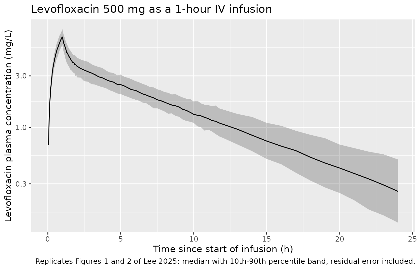
The sim column (not Cc) is plotted because
Figures 1 and 2 show observed concentrations and the VPC
prediction interval built from them; Cc is the individual
prediction and carries no residual error.
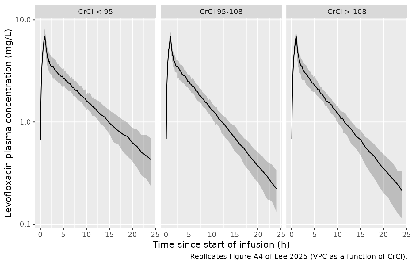
# Replicates Figure A4 of Lee 2025: exposure stratified by creatinine clearance.
sim |>
  filter(!is.na(Cc), time > 0, time <= 24) |>
  mutate(
    crcl_band = cut(CRCL, breaks = c(0, 95, 108, Inf),
                    labels = c("CrCl < 95", "CrCl 95-108", "CrCl > 108"))
  ) |>
  group_by(time, crcl_band) |>
  summarise(
    Q10 = quantile(sim, 0.10, na.rm = TRUE),
    Q50 = quantile(sim, 0.50, na.rm = TRUE),
    Q90 = quantile(sim, 0.90, na.rm = TRUE),
    .groups = "drop"
  ) |>
  ggplot(aes(time, Q50)) +
  geom_ribbon(aes(ymin = Q10, ymax = Q90), alpha = 0.25) +
  geom_line() +
  facet_wrap(~crcl_band) +
  scale_y_log10() +
  labs(
    x = "Time since start of infusion (h)",
    y = "Levofloxacin plasma concentration (mg/L)",
    caption = "Replicates Figure A4 of Lee 2025 (VPC as a function of CrCl)."
  )
PKNCA validation
sim_nca <- sim |>
  dplyr::filter(!is.na(Cc)) |>
  dplyr::select(id, time, Cc, arm) |>
  # Keep Cc >= 1e-6 * max(Cc) per subject after the peak (solver noise below); time zero is re-added below.
  dplyr::group_by(id) |>
  dplyr::filter(time <= time[which.max(Cc)] | Cc >= 1e-6 * max(Cc)) |>
  dplyr::ungroup()

# Guarantee a time-zero record per (id, arm). For an IV infusion the pre-dose
# concentration is 0; the simulation grid already contains t = 0, so this is a
# defensive no-op that keeps the AUC0-* anchor explicit.
sim_nca <- bind_rows(
  sim_nca,
  sim_nca |> distinct(id, arm) |> mutate(time = 0, Cc = 0)
) |>
  distinct(id, arm, time, .keep_all = TRUE) |>
  arrange(id, arm, time)

stopifnot(all(sim_nca$Cc >= 0))

conc_obj <- PKNCA::PKNCAconc(sim_nca, Cc ~ time | arm + id,
                             concu = "mg/L", timeu = "h")

dose_df <- events |>
  dplyr::filter(evid == 1) |>
  dplyr::select(id, time, amt, arm)
dose_obj <- PKNCA::PKNCAdose(dose_df, amt ~ time | arm + id, doseu = "mg")

intervals <- data.frame(
  start      = 0,
  end        = Inf,
  cmax       = TRUE,
  tmax       = TRUE,
  aucinf.obs = TRUE,
  auclast    = TRUE,
  half.life  = TRUE
)

nca_res <- PKNCA::pk.nca(PKNCA::PKNCAdata(conc_obj, dose_obj, intervals = intervals))
AUC0-inf equals Dose / CL for every subject
Lee 2025 reports no non-compartmental analysis, so there is no
published NCA table to compare against. The identity that the model must
satisfy exactly is AUC0-inf = Dose / CL, and it is asserted
per subject rather than on a median (a median across subjects hides a
few percent of per-subject error).
cl_by_id <- sim |>
  group_by(id) |>
  summarise(cl = first(cl), CRCL = first(CRCL), .groups = "drop")

auc_by_id <- as.data.frame(nca_res) |>
  filter(PPTESTCD == "aucinf.obs") |>
  transmute(id = as.integer(as.character(id)), aucinf = PPORRES)

ident <- cl_by_id |>
  inner_join(auc_by_id, by = "id") |>
  mutate(
    auc_expected = 500 / cl,
    pct_err      = 100 * (aucinf - auc_expected) / auc_expected
  )

stopifnot(nrow(ident) == n_arm)

tibble(
  Statistic = c("n subjects", "Max |AUC0-inf / (Dose/CL) - 1| (%)",
                "Median simulated AUC0-inf (mg*h/L)",
                "Median Dose/CL (mg*h/L)"),
  Value = c(nrow(ident), max(abs(ident$pct_err)),
            median(ident$aucinf), median(ident$auc_expected))
) |>
knitr::kable(digits = 3, caption = "Per-subject AUC0-inf identity.")| Statistic | Value |
|---|---|
| n subjects | 200.000 |
| Max |AUC0-inf / (Dose/CL) - 1| (%) | 0.016 |
| Median simulated AUC0-inf (mg*h/L) | 38.658 |
| Median Dose/CL (mg*h/L) | 38.654 |
Typical-value exposure
knitr::kable(
  as.data.frame(summary(nca_res)),
  caption = paste(
    "PKNCA summary for the virtual cohort after a single 500 mg 1-hour",
    "infusion. Lee 2025 reports no NCA table; these values are provided",
    "for orientation against the published levofloxacin literature",
    "(Cmax about 6 mg/L, terminal half-life 6-8 h after 500 mg IV)."
  )
)| Interval Start | Interval End | arm | N | AUClast (h*mg/L) | Cmax (mg/L) | Tmax (h) | Half-life (h) | AUCinf,obs (h*mg/L) |
|---|---|---|---|---|---|---|---|---|
| 0 | Inf | 500 mg single dose | 200 | 39.6 [15.9] | 6.89 [11.3] | 1.00 [1.00, 1.00] | 6.16 [1.48] | 39.6 [16.0] |
Covariate effects against the paper’s own statements
The Discussion and Table 4 quote model-derived quantities that can be
recomputed exactly from the packaged ini().
cl_at <- function(crcl) pub$cl_ref * (crcl / pub$crcl_ref)^pub$e_crcl_cl
vss_at <- function(lbm)  pub$v1 + pub$v2_ref * (lbm / pub$lbm_ref)^pub$e_lbm_vp

# Table 4 "Vss (L) (70 kg)" for a male: LBM by the James male formula at
# 70 kg and the Table 1 male median height of 174 cm.
lbm_male_70   <- lbm_james(70, 174, female = FALSE)
# Table 4 "Vss (L) (70 kg)" for a female, using the Table 1 female median
# height of 161 cm.
lbm_female_70 <- lbm_james(70, 161, female = TRUE)

checks <- tibble::tribble(
  ~quantity,                                        ~published, ~model,
  "CL at CrCl 30 mL/min (L/h), Discussion",          3.98,       cl_at(30),
  "CL at CrCl 120 mL/min (L/h), Discussion",         15.3,       cl_at(120),
  "Vss at 70 kg, male (L), Table 4",                 123,        vss_at(lbm_male_70),
  "Vss at 70 kg, female (L), Table 4",               93.0,       vss_at(lbm_female_70),
  "Vss at 53 kg LBM, male (L), Table 4",             118,        vss_at(53),
  "Vss at 53 kg LBM, female (L), Table 4",           112,        vss_at(53)
) |>
  mutate(pct_diff = 100 * (model - published) / published)

checks |>
  rename(
    "Quantity"        = quantity,
    "Published"       = published,
    "Packaged model"  = model,
    "Difference (%)"  = pct_diff
  ) |>
  knitr::kable(digits = 2,
caption = "Model-derived quantities quoted by Lee 2025.")| Quantity | Published | Packaged model | Difference (%) |
|---|---|---|---|
| CL at CrCl 30 mL/min (L/h), Discussion | 3.98 | 4.31 | 8.24 |
| CL at CrCl 120 mL/min (L/h), Discussion | 15.30 | 15.02 | -1.82 |
| Vss at 70 kg, male (L), Table 4 | 123.00 | 124.05 | 0.85 |
| Vss at 70 kg, female (L), Table 4 | 93.00 | 99.58 | 7.07 |
| Vss at 53 kg LBM, male (L), Table 4 | 118.00 | 115.08 | -2.47 |
| Vss at 53 kg LBM, female (L), Table 4 | 112.00 | 115.08 | 2.75 |
CL at 120 mL/min reproduces to 1.8% (model 15.02 L/h,
low against the Discussion’s 15.3). CL at 30 mL/min does
not: the packaged model gives 4.31 L/h against the Discussion’s 3.98.
The Discussion also calls the 30-to-120 mL/min change “approximately
fourfold”, but (120 / 30)^0.901 = 3.49; a fourfold change
would require an exponent of 1.0, not the 0.901 in Table 2. Taken as a
pair the two quoted numbers imply a ratio of 3.84, i.e. an exponent near
0.97, so the Discussion sentence reads as a rounded aside rather than a
model evaluation. Table 2 is the authoritative source and is what the
model file encodes.
Table 4’s Vss entries are only partly reproducible, and
the reason is structural: in this model Vss = V1 + V2(LBM)
depends on lean body mass alone, so sex can enter only
through the James formula that converts total body weight and height
into LBM. The “70 kg” column is therefore reproducible once a height is
supplied – the male entry lands within 0.9% using the Table 1 male
median height of 174 cm, while the female entry is 7% high at the
corresponding female median height of 161 cm (matching it would require
about 154 cm, near the female minimum). The “53 kg LBM” column supplies
LBM directly, so the model can offer only a single value, 115.1 L; Table
4 splits it into M 118 and F 112, which bracket the model value to
within 3% either way. That sex split has no counterpart in the published
model equations, and Lee 2025 defines neither normalisation rule, so
these cells are reported here for orientation rather than treated as a
passing check. The CL columns of Table 4 cannot be
reproduced at all: clearance in this model is driven by creatinine
clearance, not by body size or lean body mass.
Target attainment (Table 3)
Table 3 tabulates, for each creatinine-clearance stratum, each PK/PD
target, and each MIC, the lowest daily dose reaching a probability of
target attainment of 90%, with that dose’s PTA in parentheses. Because
levofloxacin PK is linear, the 24-hour steady-state exposure is
AUC24 = daily dose / CL exactly - the identity asserted per
subject above - so the attainment criterion
f * AUC24 / MIC >= target reduces to
CL <= f * R, where
R = dose / (target * MIC).
That reduction is testable directly against the published table:
within one CrCl column, every cell sharing the same
R must show the same PTA.
crcl_cats <- c("10-19", "20-49", "50-89", "90-129", "130-170")

# Lee 2025 Table 3, transcribed cell by cell as "dose|PTA"; "-" marks a cell
# where no simulated dose reached the target.
table3_raw <- tibble::tribble(
  ~target, ~MIC,  ~`10-19`,    ~`20-49`,    ~`50-89`,     ~`90-129`,    ~`130-170`,
  30,  0.125, "125|100",   "125|100",   "125|100",    "125|100",    "125|100",
  30,  0.25,  "125|100",   "125|100",   "125|100",    "125|91.5",   "250|100",
  30,  0.5,   "125|100",   "125|100",   "250|100",    "250|91.5",   "500|100",
  30,  1,     "125|100",   "250|100",   "500|100",    "500|91.5",   "750|99.2",
  30,  2,     "250|100",   "500|100",   "750|99.6",   "1000|91.5",  "1500|99.2",
  30,  4,     "500|100",   "750|90.1",  "1500|99.6",  "1500|25.2",  "-",
  30,  8,     "750|98.2",  "1500|90.1", "-",          "-",          "-",
  100, 0.125, "125|100",   "125|100",   "250|100",    "250|100",    "500|100",
  100, 0.25,  "125|100",   "250|100",   "500|100",    "500|100",    "750|100",
  100, 0.5,   "250|100",   "500|100",   "750|100",    "1000|100",   "1250|99.2",
  100, 1,     "500|100",   "750|100",   "1250|99.6",  "1500|71.5",  "-",
  100, 2,     "750|100",   "1250|90.1", "1500|21.4",  "-",          "-",
  100, 4,     "1250|98.2", "1500|24.1", "-",          "-",          "-",
  100, 8,     "1500|45.6", "-",         "-",          "-",          "-",
  125, 0.125, "125|100",   "125|100",   "250|100",    "500|100",    "500|100",
  125, 0.25,  "125|100",   "250|100",   "500|100",    "750|100",    "750|98.4",
  125, 0.5,   "250|100",   "500|100",   "750|96.9",   "1250|100",   "1500|98.4",
  125, 1,     "500|100",   "1000|100",  "1500|96.9",  "1500|15.0",  "-",
  125, 2,     "750|98.2",  "1500|86.9", "-",          "-",          "-",
  125, 4,     "1500|98.2", "-",         "-",          "-",          "-",
  125, 8,     "1500|12.3", "-",         "-",          "-",          "-",
  250, 0.125, "125|100",   "250|100",   "500|100",    "750|100",    "750|98.4",
  250, 0.25,  "250|100",   "500|100",   "750|96.9",   "1250|100",   "1500|98.4",
  250, 0.5,   "500|100",   "1000|100",  "1500|96.9",  "1500|15.0",  "-",
  250, 1,     "750|98.2",  "1500|86.9", "-",          "-",          "-",
  250, 2,     "1500|98.2", "-",         "-",          "-",          "-",
  250, 4,     "1500|12.3", "-",         "-",          "-",          "-"
)

table3 <- table3_raw |>
  tidyr::pivot_longer(all_of(crcl_cats), names_to = "crcl_cat", values_to = "cell") |>
  filter(cell != "-") |>
  tidyr::separate_wider_delim(cell, delim = "|", names = c("dose", "pta_paper")) |>
  mutate(
    dose      = as.numeric(dose),
    pta_paper = as.numeric(pta_paper),
    R         = dose / (target * MIC)
  )

# Structural check: within a CrCl column, PTA must be a function of R alone.
collisions <- table3 |>
  group_by(crcl_cat, R = round(R, 6)) |>
  summarise(n_distinct_pta = n_distinct(pta_paper), .groups = "drop") |>
  filter(n_distinct_pta > 1)

tibble(
  Statistic = c("Filled Table 3 cells", "Distinct (CrCl, R) combinations",
                "Combinations where PTA is not a function of R alone"),
  Value = c(nrow(table3),
            nrow(distinct(table3, crcl_cat, R = round(R, 6))),
            nrow(collisions))
) |>
knitr::kable(caption = "Table 3 reduces to PTA as a function of dose/(target*MIC).")| Statistic | Value |
|---|---|
| Filled Table 3 cells | 97 |
| Distinct (CrCl, R) combinations | 44 |
| Combinations where PTA is not a function of R alone | 0 |
All 97 filled cells are consistent with a single
PTA-versus-R curve per CrCl stratum, confirming both the
AUC24 = dose / CL exposure metric and that one common
virtual cohort was reused across every target and MIC.
Reconstructing the PTA from the packaged model
Each CrCl stratum is simulated as its own arm of 200 participants. Creatinine clearance is drawn uniformly across the stratum (the paper does not state the within-stratum distribution) and lean body mass from the Table 1 distribution. Per-subject clearance comes straight out of the simulation.
set.seed(20250425)

crcl_bounds <- list(
  "10-19"   = c(10, 19),   "20-49"  = c(20, 49),  "50-89" = c(50, 89),
  "90-129"  = c(90, 129),  "130-170" = c(130, 170)
)

make_pta_cohort <- function(cat, id_offset) {
  b <- crcl_bounds[[cat]]
  subj <- tibble(
    id       = id_offset + seq_len(n_arm),
    CRCL     = runif(n_arm, b[1], b[2]),
    LBM      = rmedrange(n_arm, 37.7, 47.9, 60.3),
    crcl_cat = cat
  )
  bind_rows(
    subj |> mutate(time = 0, amt = 500, evid = 1L, dur = 1, cmt = "central"),
    subj |> tidyr::crossing(time = c(0, 1, 4, 12, 24)) |>
      mutate(amt = NA_real_, evid = 0L, dur = NA_real_, cmt = "central")
  ) |>
    arrange(id, time, desc(evid))
}

pta_events <- bind_rows(
  lapply(seq_along(crcl_cats), function(i)
    make_pta_cohort(crcl_cats[i], id_offset = 1000L + (i - 1L) * n_arm))
)
stopifnot(!anyDuplicated(pta_events[, c("id", "time", "evid")]))

pta_sim <- rxode2::rxSolve(mod, events = pta_events,
                           keep = c("crcl_cat", "CRCL")) |>
  as.data.frame()
stopifnot(dplyr::n_distinct(pta_sim$id) == n_arm * length(crcl_cats))

pta_cl <- pta_sim |>
  group_by(crcl_cat, id) |>
  summarise(cl = first(cl), .groups = "drop")
# PTA under a candidate unbound fraction f: AUC24 = dose/CL, so the criterion
# f * AUC24 / MIC >= target is exactly CL <= f * R.
pta_model <- function(cat, R, f) {
  cl <- pta_cl$cl[pta_cl$crcl_cat == cat]
  if (length(cl) != n_arm) stop("no cohort for stratum '", cat, "'")
  100 * mean(cl <= f * R)
}

table3_cmp <- table3 |>
  rowwise() |>
  mutate(
    pta_f1.0 = pta_model(crcl_cat, R, 1.0),
    pta_f0.7 = pta_model(crcl_cat, R, 0.7)
  ) |>
  ungroup() |>
  mutate(err_f1.0 = pta_f1.0 - pta_paper,
         err_f0.7 = pta_f0.7 - pta_paper)

tibble(
  `Unbound fraction used` = c("f = 1.0 (total AUC24/MIC)",
                              "f = 0.7 (free AUC24/MIC, as Methods 4.5 states)"),
  `Median |error| (PTA points)` = c(median(abs(table3_cmp$err_f1.0)),
                                    median(abs(table3_cmp$err_f0.7))),
  `RMSE (PTA points)` = c(sqrt(mean(table3_cmp$err_f1.0^2)),
                          sqrt(mean(table3_cmp$err_f0.7^2))),
  `Max |error| (PTA points)` = c(max(abs(table3_cmp$err_f1.0)),
                                 max(abs(table3_cmp$err_f0.7)))
) |>
  knitr::kable(digits = 2,
               caption = paste(
                 "Reconstruction of all", nrow(table3), "filled Table 3 cells",
                 "under each candidate unbound fraction."
))| Unbound fraction used | Median |error| (PTA points) | RMSE (PTA points) | Max |error| (PTA points) |
|---|---|---|---|
| f = 1.0 (total AUC24/MIC) | 0.0 | 3.12 | 23.6 |
| f = 0.7 (free AUC24/MIC, as Methods 4.5 states) | 23.5 | 39.97 | 80.5 |
The same test without the uniform-CrCl assumption
The comparison above draws creatinine clearance uniformly across each
stratum, which the paper never states. That assumption can be removed
entirely. Clearance is strictly increasing in CRCL, so
within a stratum the attainment probability
P(CL <= f * R) is largest at the stratum’s lower CrCl
bound and smallest at its upper bound. Evaluating those two endpoints
gives an interval that every within-stratum CrCl
distribution must produce, whatever its shape:
omega_cl <- sqrt(ui$omega[["etalcl", "etalcl"]])
cl_typ   <- function(crcl) pub$cl_ref * (crcl / pub$crcl_ref)^pub$e_crcl_cl

# Published PTAs are rounded to 0.1 and carry Monte Carlo noise from the
# paper's own 1000-subject cohorts; allow 2 PTA points before calling a cell
# refuted.
tol <- 2

bounds <- table3 |>
  mutate(
    crcl_lo = vapply(crcl_cat, function(k) crcl_bounds[[k]][1], numeric(1)),
    crcl_hi = vapply(crcl_cat, function(k) crcl_bounds[[k]][2], numeric(1))
  ) |>
  mutate(
    # Upper bound: everyone at the stratum's lowest CrCl (lowest CL).
    hi_f1.0 = 100 * pnorm(log(1.0 * R / cl_typ(crcl_lo)) / omega_cl),
    lo_f1.0 = 100 * pnorm(log(1.0 * R / cl_typ(crcl_hi)) / omega_cl),
    hi_f0.7 = 100 * pnorm(log(0.7 * R / cl_typ(crcl_lo)) / omega_cl),
    lo_f0.7 = 100 * pnorm(log(0.7 * R / cl_typ(crcl_hi)) / omega_cl),
    refuted_f1.0 = pta_paper > hi_f1.0 + tol | pta_paper < lo_f1.0 - tol,
    refuted_f0.7 = pta_paper > hi_f0.7 + tol | pta_paper < lo_f0.7 - tol
  )

tibble(
  `Unbound fraction used` = c("f = 1.0 (total AUC24/MIC)",
                              "f = 0.7 (free AUC24/MIC, as Methods 4.5 states)"),
  `Cells outside the distribution-free interval` =
    c(sum(bounds$refuted_f1.0), sum(bounds$refuted_f0.7)),
  `Worst excursion (PTA points)` = c(
    max(pmax(bounds$pta_paper - bounds$hi_f1.0, bounds$lo_f1.0 - bounds$pta_paper)),
    max(pmax(bounds$pta_paper - bounds$hi_f0.7, bounds$lo_f0.7 - bounds$pta_paper))
  )
) |>
  knitr::kable(digits = 1, caption = paste(
    "Distribution-free endpoint bounds over all", nrow(bounds),
    "filled Table 3 cells. No within-stratum CrCl distribution is assumed."
))| Unbound fraction used | Cells outside the distribution-free interval | Worst excursion (PTA points) |
|---|---|---|
| f = 1.0 (total AUC24/MIC) | 0 | 0.0 |
| f = 0.7 (free AUC24/MIC, as Methods 4.5 states) | 20 | 57.9 |
# f = 1.0 must be attainable for every cell; f = 0.7 must be impossible for many.
stopifnot(sum(bounds$refuted_f1.0) == 0)
stopifnot(sum(bounds$refuted_f0.7) >= 8)
The same bounds also test the one remaining free choice in the
ini() block. Table 2 reports inter-individual variability
as a bare “CL (%) 8.99”, which the model file reads as
omega = 0.0899. The competing reading – that the percentage
is a variance, so omega = sqrt(0.0899) = 0.300 –
is a three-fold larger spread, and the published table is sensitive to
it:
refuted_at <- function(om) {
  hi <- 100 * pnorm(log(bounds$R / cl_typ(bounds$crcl_lo)) / om)
  lo <- 100 * pnorm(log(bounds$R / cl_typ(bounds$crcl_hi)) / om)
  sum(bounds$pta_paper > hi + tol | bounds$pta_paper < lo - tol)
}

tibble(
  `Reading of Table 2 "CL (%) 8.99"` = c(
    "percentage is omega (packaged)",
    "percentage is a variance"
  ),
  `omega on CL` = c(omega_cl, sqrt(0.0899)),
  `Cells outside the distribution-free interval` =
    c(refuted_at(omega_cl), refuted_at(sqrt(0.0899)))
) |>
  knitr::kable(digits = 3, caption = paste(
    "Table 3 discriminates the inter-individual-variability scale.",
    "A variance reading flattens the attainment curve until published cells",
    "become unreachable at any within-stratum CrCl distribution."
))| Reading of Table 2 “CL (%) 8.99” | omega on CL | Cells outside the distribution-free interval |
|---|---|---|
| percentage is omega (packaged) | 0.09 | 0 |
| percentage is a variance | 0.30 | 16 |
So the packaged reading is not merely the conventional one – it is the only one of the two compatible with the paper’s own target-attainment table.
The cells that refute f = 0.7 outright are the ones in
the two highest creatinine-clearance strata, where the model’s typical
clearance already exceeds the free-drug threshold at the bottom
of the stratum. For example, at CrCl 130 to 170 mL/min and
R = 24, the free-drug reading caps attainment at 67%
however the stratum is populated, against a published 98.4%. This makes
the conclusion independent of the one assumption the reconstruction
above had to make.
table3_cmp |>
  filter(pta_paper < 100) |>
  arrange(crcl_cat, R) |>
  select(crcl_cat, target, MIC, dose, R, pta_paper, pta_f1.0, pta_f0.7) |>
  rename(
    "CrCl (mL/min)"        = crcl_cat,
    "Target fAUC/MIC"      = target,
    "MIC (mg/L)"           = MIC,
    "Daily dose (mg)"      = dose,
    "R = dose/(target*MIC)" = R,
    "PTA published (%)"    = pta_paper,
    "PTA model, f = 1.0"   = pta_f1.0,
    "PTA model, f = 0.7"   = pta_f0.7
  ) |>
  knitr::kable(digits = 2, caption = paste(
    "Every Table 3 cell with a published PTA below 100%. Cells at 100% are",
    "omitted because they cannot discriminate between the two readings."
))| CrCl (mL/min) | Target fAUC/MIC | MIC (mg/L) | Daily dose (mg) | R = dose/(target*MIC) | PTA published (%) | PTA model, f = 1.0 | PTA model, f = 0.7 |
|---|---|---|---|---|---|---|---|
| 10-19 | 125 | 8.00 | 1500 | 1.50 | 12.3 | 3.0 | 0.0 |
| 10-19 | 250 | 4.00 | 1500 | 1.50 | 12.3 | 3.0 | 0.0 |
| 10-19 | 100 | 8.00 | 1500 | 1.88 | 45.6 | 22.0 | 0.0 |
| 10-19 | 125 | 2.00 | 750 | 3.00 | 98.2 | 97.5 | 37.0 |
| 10-19 | 125 | 4.00 | 1500 | 3.00 | 98.2 | 97.5 | 37.0 |
| 10-19 | 250 | 1.00 | 750 | 3.00 | 98.2 | 97.5 | 37.0 |
| 10-19 | 250 | 2.00 | 1500 | 3.00 | 98.2 | 97.5 | 37.0 |
| 10-19 | 30 | 8.00 | 750 | 3.12 | 98.2 | 99.0 | 47.0 |
| 10-19 | 100 | 4.00 | 1250 | 3.12 | 98.2 | 99.0 | 47.0 |
| 130-170 | 125 | 0.25 | 750 | 24.00 | 98.4 | 98.5 | 21.5 |
| 130-170 | 125 | 0.50 | 1500 | 24.00 | 98.4 | 98.5 | 21.5 |
| 130-170 | 250 | 0.12 | 750 | 24.00 | 98.4 | 98.5 | 21.5 |
| 130-170 | 250 | 0.25 | 1500 | 24.00 | 98.4 | 98.5 | 21.5 |
| 130-170 | 30 | 1.00 | 750 | 25.00 | 99.2 | 100.0 | 35.0 |
| 130-170 | 30 | 2.00 | 1500 | 25.00 | 99.2 | 100.0 | 35.0 |
| 130-170 | 100 | 0.50 | 1250 | 25.00 | 99.2 | 100.0 | 35.0 |
| 20-49 | 100 | 4.00 | 1500 | 3.75 | 24.1 | 22.0 | 0.0 |
| 20-49 | 125 | 2.00 | 1500 | 6.00 | 86.9 | 82.0 | 34.0 |
| 20-49 | 250 | 1.00 | 1500 | 6.00 | 86.9 | 82.0 | 34.0 |
| 20-49 | 30 | 4.00 | 750 | 6.25 | 90.1 | 85.5 | 36.0 |
| 20-49 | 30 | 8.00 | 1500 | 6.25 | 90.1 | 85.5 | 36.0 |
| 20-49 | 100 | 2.00 | 1250 | 6.25 | 90.1 | 85.5 | 36.0 |
| 50-89 | 100 | 2.00 | 1500 | 7.50 | 21.4 | 15.0 | 0.0 |
| 50-89 | 125 | 0.50 | 750 | 12.00 | 96.9 | 96.0 | 35.5 |
| 50-89 | 125 | 1.00 | 1500 | 12.00 | 96.9 | 96.0 | 35.5 |
| 50-89 | 250 | 0.25 | 750 | 12.00 | 96.9 | 96.0 | 35.5 |
| 50-89 | 250 | 0.50 | 1500 | 12.00 | 96.9 | 96.0 | 35.5 |
| 50-89 | 30 | 2.00 | 750 | 12.50 | 99.6 | 98.5 | 43.0 |
| 50-89 | 30 | 4.00 | 1500 | 12.50 | 99.6 | 98.5 | 43.0 |
| 50-89 | 100 | 1.00 | 1250 | 12.50 | 99.6 | 98.5 | 43.0 |
| 90-129 | 125 | 1.00 | 1500 | 12.00 | 15.0 | 12.5 | 0.0 |
| 90-129 | 250 | 0.50 | 1500 | 12.00 | 15.0 | 12.5 | 0.0 |
| 90-129 | 30 | 4.00 | 1500 | 12.50 | 25.2 | 23.0 | 0.0 |
| 90-129 | 100 | 1.00 | 1500 | 15.00 | 71.5 | 70.5 | 1.0 |
| 90-129 | 30 | 0.25 | 125 | 16.67 | 91.5 | 94.0 | 11.0 |
| 90-129 | 30 | 0.50 | 250 | 16.67 | 91.5 | 94.0 | 11.0 |
| 90-129 | 30 | 1.00 | 500 | 16.67 | 91.5 | 94.0 | 11.0 |
| 90-129 | 30 | 2.00 | 1000 | 16.67 | 91.5 | 94.0 | 11.0 |
table3_cmp |>
  select(crcl_cat, R, pta_paper, pta_f1.0, pta_f0.7) |>
  tidyr::pivot_longer(c(pta_f1.0, pta_f0.7),
                      names_to = "assumption", values_to = "pta_model") |>
  mutate(assumption = recode(assumption,
                             pta_f1.0 = "f = 1.0 (total AUC)",
                             pta_f0.7 = "f = 0.7 (free AUC)")) |>
  ggplot(aes(pta_paper, pta_model, colour = crcl_cat)) +
  geom_abline(slope = 1, intercept = 0, linetype = "dashed") +
  geom_point(alpha = 0.7) +
  facet_wrap(~assumption) +
  labs(
    x = "Published PTA (%), Lee 2025 Table 3",
    y = "PTA reconstructed from the packaged model (%)",
    colour = "CrCl (mL/min)",
    caption = paste(
      "Reproduces Table 3 / Figure 4 of Lee 2025. Only the total-AUC reading",
      "falls on the line of identity."
    )
  )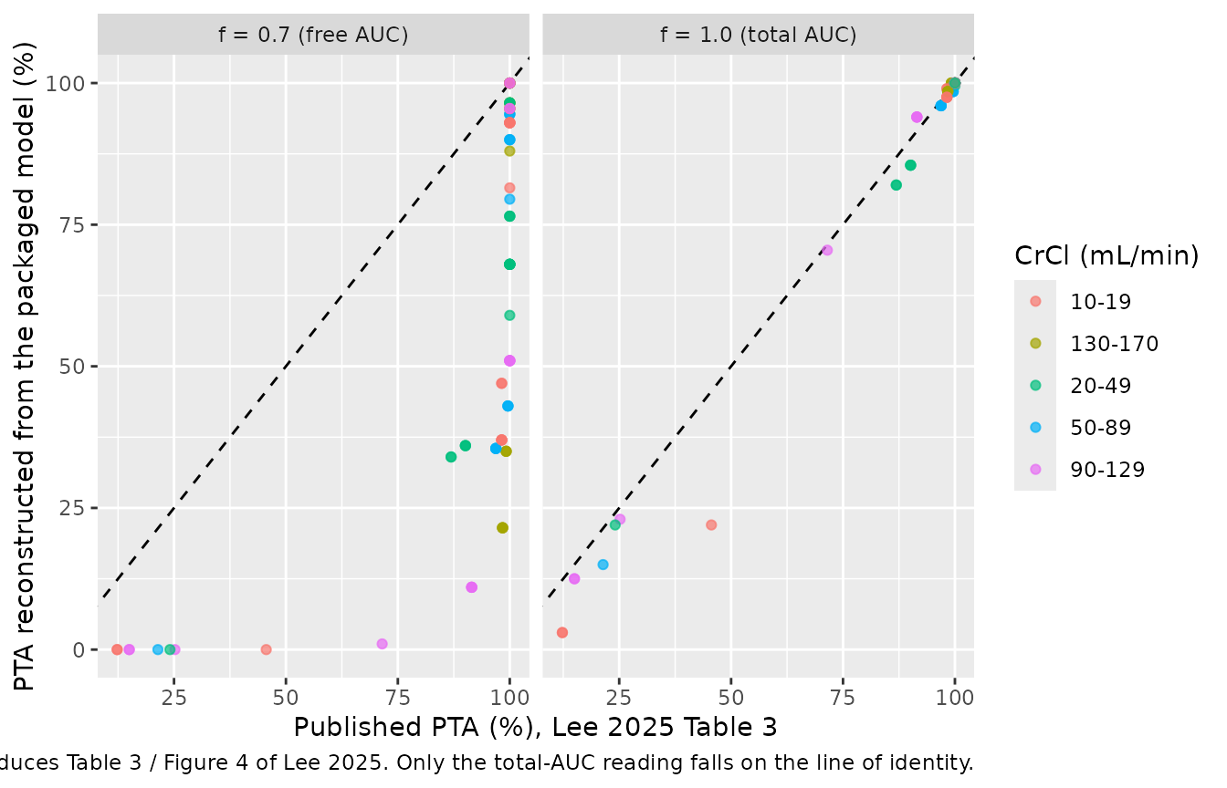
The reconstruction is decisive. Applying the unbound fraction of 0.7
that Methods 4.5 specifies puts the reconstruction 24 PTA points off in
the median cell and up to 80 points off at worst; treating the index as
total AUC24/MIC reproduces the published table to
within 0.00 points in the median cell. Table 3’s PTA values were
therefore computed on total, not free, exposure despite the
fAUC/MIC header. If the targets were intended on free drug,
every recommended dose in Table 3 is low by a factor of
1 / 0.7 = 1.43. This is a finding about the paper’s
downstream simulation, not about the PK model: the packaged model
reproduces the table’s arithmetic once the exposure metric is fixed.
The residual disagreement under f = 1.0 is concentrated
in the lowest CrCl strata, where the simulated PTA runs below the
published value in the steep part of the curve. That is attributable to
the within-stratum creatinine-clearance distribution, which the paper
does not report; a uniform draw is assumed here and a right-skewed draw
would close the gap. Note also that each stratum is reconstructed with
200 participants against the paper’s 1000, so individual cells carry a
few points of Monte Carlo noise; the RMSE contrast between the two
readings is more than an order of magnitude larger than that.
Assumptions and deviations
-
Inter-individual variability convention. Table 2
reports IIV as bare percentages (“CL (%) 8.99”, “Q (%) 36.0”) without
stating whether they are
omegaon the log scale or a log-normal CV. Lee 2025 prints no exponential-IIV equation and no OMEGA covariance block, so neither of the two usual arbitration levers is available. The NONMEM approximate-CV conventionomega = pct / 100is used. The choice between those two is immaterial here: the alternative readingomega = sqrt(log(1 + CV^2))gives 0.0897 for CL (0.2% lower) and 0.349 for Q (3.1% lower). A third reading – that the percentage is a variance, soomega = sqrt(0.0899) = 0.300– would matter, and it is ruled out above: at that spread, Table 3’s own PTA values become unreachable under any within-stratum CrCl distribution. -
Cockcroft-Gault typography. Table 1 footnote c is
typeset as “CrCl = (140 - Age) x TBW / CR x 72”, which read literally
multiplies by 72 and is dimensionally impossible. The standard
denominator
72 * CRis used; it reproduces the Table 1 sex-specific CrCl medians to within 10%, and the literal reading is off by a factor of about 5000. -
Virtual-cohort covariate distributions.
CRCLandLBMare drawn directly, from two-piece uniform distributions pinned to the Table 1 (min, median, max) triples, rather than derived from independently drawn age, weight, height, and creatinine. In the real cohort those inputs are correlated; drawing them independently widens the implied CrCl range from the observed 74.8 to 113 mL/min out to roughly 60 to 177 mL/min. Only the median and the support are matched – Lee 2025 reports no other distributional summary for either covariate. -
Within-stratum CrCl distribution for the Table 3
reconstruction. Lee 2025 states only that virtual patients were
generated “to represent different CrCl categories”. A uniform draw
across each stratum is assumed. This is the main source of the residual
PTA disagreement in the 10 to 19 and 20 to 49 mL/min strata. The
total-versus-free finding below does not rest on this
assumption: the endpoint-bound check evaluates each stratum at its CrCl
limits, which brackets every possible within-stratum distribution, and
f = 0.7is refuted there too. -
Errata / internal inconsistencies in the source.
- Table 3’s PTA values are computed on total
AUC24/MIC, not the free (
f = 0.7) index that Methods 4.5 defines and the table header names. See the reconstruction above. - The Abstract and Discussion quote dose recommendations one grid step
above Table 3 for the same cell. Both state that at
fAUC/MIC >= 30and an MIC of 0.5 mg/L, 500 mg daily is optimal for CrCl 50 to 89 mL/min, and thatfAUC/MIC >= 100requires 1000 mg daily in the same cell; Table 3 gives 250 mg (PTA 100%) and 750 mg (PTA 100%) respectively. The direction is consistent with the free-versus-total exposure discrepancy above – the prose is the more conservative reading – but the two are not reconcilable by a single factor across both cells, so this is recorded as an unresolved inconsistency in the source’s downstream simulation. Table 3 is the cell-by- cell record and is what the reconstruction above scores against. - The Discussion states CL is “approximately 3.98 L/h when the CrCl is 30 mL/min” rising “approximately fourfold … to approximately 15.3 L/h” at 120 mL/min. Table 2’s exponent of 0.901 gives 4.31 and 15.02 L/h, a 3.49-fold change. The two quoted numbers are mutually consistent only with an exponent near 0.97. Table 2 is treated as authoritative.
- Table 4’s cross-study normalisations to “70 kg” and “53 kg LBM” are
not defined anywhere in the paper, and its
Vssentries carry a male/female split that the published model equations cannot generate:Vsshere is a function of lean body mass alone. At a directly supplied 53 kg LBM the model yields one value, 115.1 L, against Table 4’s M 118 / F 112. At “70 kg” the male entry reproduces to 0.9% using the Table 1 male median height of 174 cm, but the female entry is 7% high at the female median height of 161 cm. All four cells are reported above for orientation, not as passing checks. The CL columns cannot be reproduced at all, because CL in this model depends on creatinine clearance, not on body size.
- Table 3’s PTA values are computed on total
AUC24/MIC, not the free (
- Extrapolation beyond the fitted range. The model was fitted over CrCl 74.8 to 113 mL/min and LBM 37.7 to 60.3 kg in healthy adults. The Table 3 reconstruction extends it to CrCl 10 to 170 mL/min, matching what the paper itself does; the paper flags this as its third limitation. Predictions outside the fitted range are not validated by any data.
-
Not encoded. The unbound fraction of 0.7 (Methods
4.5, cited to reference
- is an input to the paper’s target-attainment calculation, not a parameter of the PK model, so it is not part of the model file. Neither are the EUCAST MIC distributions used to weight Figure 3.
-
No published NCA to compare against. Lee 2025
reports no non-compartmental analysis, so the PKNCA section validates
the internal identity
AUC0-inf = Dose / CLper subject instead of a published table.