Targeted therapies in systemic sclerosis, mRSS and FVC MBMA (Vaskeikina 2026)
Source:vignettes/articles/Vaskeikina_2026_systemicSclerosis.Rmd
Vaskeikina_2026_systemicSclerosis.RmdModel and source
mod <- rxode2::rxode2(readModelDb("Vaskeikina_2026_systemicSclerosis_mbma"))
#> ℹ parameter labels from comments will be replaced by 'label()'
Citation: Vaskeikina M, Ugolkov Y, Kireev B, Peskov K, Volkova A. Systematic Review and Model-Based Meta-Analysis of Targeted Drugs for Systemic Sclerosis. Pharmaceutics. 2026;18(2):250. doi:10.3390/pharmaceutics18020250.
Description: MBMA. Longitudinal model-based meta-analysis of targeted therapies in systemic sclerosis (SSc), fit in Monolix 2024R1 to study-arm-level aggregate data from 32 randomized controlled trials (73 arms, 2036 patients, 23 targeted agents). Two endpoints are modelled jointly as change from baseline: the modified Rodnan skin score (mrsscfb, points; 30 trials) and percent-predicted forced vital capacity (fvcppcfb, % predicted; 20 trials). Each follows an Emax-in-time function CFB(t) = Emax * t / (ET50 + t) with ONE shared ET50 of 27.49 weeks. The arm Emax is the comparator (standard-of-care) typical value plus an ADDITIVE per-drug shift for the six drugs with a distinguishable mRSS effect (abatacept, baricitinib, guselkumab, inebilizumab, rituximab, tofacitinib) and the four with a distinguishable FVC effect (belimumab, nintedanib, rituximab, tocilizumab), selected by the TRT_
arm indicators. Variability is two-level and additive on Emax: between-study (eta_study_) and between-treatment-arm (eta_arm_), the latter and the residual both divided by sqrt(N_ARM), the arm sample size, which is therefore a required input column. No baseline covariate was retained. Suitable for simulating study-arm-mean change-from-baseline trajectories, NOT individual-patient scores.
This is a model-based meta-analysis (MBMA): every modelled data point is a study-arm mean change from baseline, not a patient. Two endpoints are modelled jointly and share one time to half-maximal response:
-
mrsscfb, the change from baseline in the modified Rodnan skin score (mRSS, 17 sites scored 0-3, so 0-51 points; a fall is an improvement), and -
fvcppcfb, the change from baseline in forced vital capacity as a percentage of the predicted value (a rise is an improvement).
Population
| Field | Value |
|---|---|
| species | human |
| n_subjects | 2036 |
| n_studies | 32 |
| n_arms | 73 |
| age_range | study-arm means; overall mean age 50.5 years (Section 3.1) |
| weight_range | not reported |
| sex_female_pct | 75.5 |
| race_ethnicity | collected per arm but not reported in the publication |
| disease_state | adults with systemic sclerosis enrolled in randomized controlled trials of targeted therapies: diffuse cutaneous SSc in 16 studies, unspecified SSc in 11, SSc-associated pulmonary arterial hypertension in 1 (excluded from modelling because it reported neither mRSS nor FVC); only 4 studies explicitly reported interstitial lung disease |
| dose_range | not modelled; every dose arm of a drug is pooled into a single per-drug effect |
| regimens | 23 targeted agents (cytokine, surface-receptor, intracellular-kinase and antifibrotic targets) versus a standard-of-care comparator arm |
| baseline_scores | across-study mean baseline mRSS 22.2 points and percent-predicted FVC 83.4% (Section 3.1) |
| timepoints | follow-up up to about two years; 16 of 30 mRSS trials and 14 of 20 FVC trials contributed a single post-baseline assessment (Section 3.1) |
| regions | not reported |
| notes | MBMA at the study-arm level. mRSS was modelled from 30 trials and percent-predicted FVC from 20 (21 reported FVC; STRATUS was excluded because its mL values could not be converted to percent predicted). Arm means and SDs were harmonised from medians, IQRs, SEs and CIs with published conversion formulas, and data were digitised from figures with PlotDigitizer. The model simulates arm-mean change-from-baseline trajectories and is NOT suitable for individual-subject simulation. |
Vaskeikina 2026 searched PubMed and ClinicalTrials.gov (PRISMA, registered on OSF) for randomized controlled trials of targeted therapies in SSc. Of 267 records, 32 trials met the criteria (Section 3.1, Figure 1): 73 arms, 2036 patients, mean age 50.5 years and 75.5% women. Across studies the mean baseline mRSS was 22.2 points and the mean baseline FVC was 83.4% of predicted. mRSS was modelled from 30 trials and percent-predicted FVC from 20.
Source trace
Every ini() value is from Table 1
(“Parameter estimates of final longitudinal MBMA model”). The equations
are the numbered display equations of Section 2.3 and 2.4.
| Quantity | Model file | Source location | Value |
|---|---|---|---|
| Time course | tcourse, mrsscfb, fvcppcfb | Eq. 8 | CFB(t) = Emax * t / (ET50 + t) |
| Residual error | addSd_ | Eq. 9 | eps ~ N(0, sigma^2 / N) |
| Random effects on Emax | eta_study_, eta_arm_ / sqrt(N_ARM) | Eq. 10 | BSV ~ N(0, omega^2); BTAV ~ N(0, gamma^2 / N) |
| Treatment effects | e_trt_ |
Eq. 11 | Emaxpop + sum(beta_TRT) + BSV + BTAV |
| Comparator mRSS Emax | emax_mrss | Table 1 | -5.29 points (RSE 22.2%) |
| Abatacept, mRSS | e_trt_abatacept_emax_mrss | Table 1 | -5.41 (RSE 44.6%) |
| Baricitinib, mRSS | e_trt_baricitinib_emax_mrss | Table 1 | -13.87 (RSE 35.4%) |
| Guselkumab, mRSS | e_trt_guselkumab_emax_mrss | Table 1 | -23.55 (RSE 16.7%) |
| Inebilizumab, mRSS | e_trt_inebilizumab_emax_mrss | Table 1 | -13.45 (RSE 38.0%) |
| Rituximab, mRSS | e_trt_rituximab_emax_mrss | Table 1 | -8.03 (RSE 26.3%) |
| Tofacitinib, mRSS | e_trt_tofacitinib_emax_mrss | Table 1 | -14.35 (RSE 18.4%) |
| BSV, mRSS Emax | eta_study_emax_mrss | Table 1 | SD 4.53 (RSE 19.6%) |
| BTAV, mRSS Emax | eta_arm_emax_mrss | Table 1 | SD 10.23 (RSE 28.7%) |
| Residual, mRSS | addSd_mrsscfb | Table 1 | SD 4.12 (RSE 10.0%) |
| Comparator FVC Emax | emax_fvc | Table 1 | -2.29 % predicted (RSE 35.3%) |
| Nintedanib, FVC | e_trt_nintedanib_emax_fvc | Table 1 | 2.06 (RSE 45.5%) |
| Rituximab, FVC | e_trt_rituximab_emax_fvc | Table 1 | 9.81 (RSE 20.1%) |
| Tocilizumab, FVC | e_trt_tocilizumab_emax_fvc | Table 1 | 4.49 (RSE 31.7%) |
| Belimumab, FVC | e_trt_belimumab_emax_fvc | Table 1 | 10.38 (RSE 43.0%) |
| BSV, FVC Emax | eta_study_emax_fvc | Table 1 | SD 1.97 (RSE 38.0%) |
| BTAV, FVC Emax | eta_arm_emax_fvc | Table 1 | SD 9.94 (RSE 30.1%) |
| Residual, FVC | addSd_fvcppcfb | Table 1 | SD 4.42 (RSE 12.0%) |
| Shared ET50 | let50 | Table 1 | 27.49 weeks (RSE 16.6%) |
The packaged values are checked against Table 1 here, so a
mis-transcription cannot pass silently. Table 1 labels every random
effect and residual as a “Standard deviation”, so ini()
holds their squares.
published <- c(
  emax_mrss = -5.29,
  e_trt_abatacept_emax_mrss = -5.41,
  e_trt_baricitinib_emax_mrss = -13.87,
  e_trt_guselkumab_emax_mrss = -23.55,
  e_trt_inebilizumab_emax_mrss = -13.45,
  e_trt_rituximab_emax_mrss = -8.03,
  e_trt_tofacitinib_emax_mrss = -14.35,
  emax_fvc = -2.29,
  e_trt_nintedanib_emax_fvc = 2.06,
  e_trt_rituximab_emax_fvc = 9.81,
  e_trt_tocilizumab_emax_fvc = 4.49,
  e_trt_belimumab_emax_fvc = 10.38,
  let50 = log(27.49),
  addSd_mrsscfb = 4.12,
  addSd_fvcppcfb = 4.42
)
theta <- mod$theta
stopifnot(
  setequal(names(theta), names(published)),
  isTRUE(all.equal(theta[names(published)], published, tolerance = 1e-12))
)

omega_sd <- sqrt(diag(mod$omega))
stopifnot(isTRUE(all.equal(
  omega_sd[c("eta_study_emax_mrss", "eta_arm_emax_mrss", "eta_study_emax_fvc", "eta_arm_emax_fvc")],
  c(eta_study_emax_mrss = 4.53, eta_arm_emax_mrss = 10.23, eta_study_emax_fvc = 1.97, eta_arm_emax_fvc = 9.94),
  tolerance = 1e-12
)))
The paper converts the shared ET50 into months in the Abstract (“a 6.3-month period for half treatment response development”):
Structural model
For endpoint a in study i, treatment arm k
with N participants and follow-up time t in weeks
(Equations 8-11):
Two features are specific to the meta-analytic setting, and both are
why the arm size is a model input (N_ARM)
rather than a scaling applied after the solve: the between-arm random
effect is divided by sqrt(N), and so is the residual. A
per-arm random-effect SD cannot be varied across arms within one
rxSolve() without a data column.
Treatment enters only through the TRT_<DRUG> arm
indicators: there is no dose or exposure term, and every dose arm of a
drug is pooled into one effect. A comparator arm has all nine indicators
set to 0.
Building an event table
The model has no ODE state and two observation endpoints, so
observation rows are tagged by dvid (1 =
mrsscfb, 2 = fvcppcfb) with no
cmt. Each id is one study arm.
trt_cols <- c(
  "TRT_ABATACEPT", "TRT_BARICITINIB", "TRT_GUSELKUMAB", "TRT_INEBILIZUMAB",
  "TRT_RITUXIMAB", "TRT_TOFACITINIB", "TRT_BELIMUMAB", "TRT_NINTEDANIB",
  "TRT_TOCILIZUMAB"
)

# arms: one row per arm with columns id, N_ARM and any TRT_<DRUG> set to 1.
make_events <- function(arms, times) {
  ev <- tidyr::expand_grid(arms, time = times, dvid = 1:2)
  for (nm in setdiff(trt_cols, names(ev))) ev[[nm]] <- 0
  ev |>
    mutate(evid = 0L, cmt = NA_integer_) |>
    arrange(id, time, dvid) |>
    as.data.frame()
}
Validation
There is no drug concentration in this model, so a PKNCA non-compartmental analysis does not apply; the checks below are closed-form and simulation checks of the change-from-baseline endpoints.
Closed-form gate
The model is algebraic, so it can be checked against an independent R implementation of Equations 8-11 evaluated at the same drawn random effects. Both sides use identical parameters, so the only difference is numerical and a tight bound is the right assertion.
rxode2::rxSetSeed(20261015)

arm_design <- tibble(
  label = c("comparator", "abatacept", "baricitinib", "guselkumab", "inebilizumab",
            "rituximab", "tofacitinib", "belimumab", "nintedanib", "tocilizumab"),
  drug_col = c(NA, "TRT_ABATACEPT", "TRT_BARICITINIB", "TRT_GUSELKUMAB", "TRT_INEBILIZUMAB",
               "TRT_RITUXIMAB", "TRT_TOFACITINIB", "TRT_BELIMUMAB", "TRT_NINTEDANIB",
               "TRT_TOCILIZUMAB")
)
arms_cf <- arm_design |>
  tidyr::expand_grid(N_ARM = c(8, 15, 46, 120, 288)) |>
  mutate(id = row_number())
for (nm in trt_cols) arms_cf[[nm]] <- as.numeric(arms_cf$drug_col %in% nm)

sim_cf <- rxode2::rxSolve(mod, make_events(arms_cf |> select(-label, -drug_col), c(0, 4, 12, 24, 52, 104)))

etas <- as.data.frame(sim_cf$params)[, c("id", "eta_study_emax_mrss", "eta_arm_emax_mrss",
                                        "eta_study_emax_fvc", "eta_arm_emax_fvc")]
etas$id <- as.integer(as.character(etas$id))

p <- published
closed <- as.data.frame(sim_cf) |>
  mutate(id = as.integer(id)) |>
  left_join(etas, by = "id") |>
  mutate(
    f = time / (exp(p[["let50"]]) + time),
    emax_mrss_ref = p[["emax_mrss"]] +
      p[["e_trt_abatacept_emax_mrss"]] * TRT_ABATACEPT +
      p[["e_trt_baricitinib_emax_mrss"]] * TRT_BARICITINIB +
      p[["e_trt_guselkumab_emax_mrss"]] * TRT_GUSELKUMAB +
      p[["e_trt_inebilizumab_emax_mrss"]] * TRT_INEBILIZUMAB +
      p[["e_trt_rituximab_emax_mrss"]] * TRT_RITUXIMAB +
      p[["e_trt_tofacitinib_emax_mrss"]] * TRT_TOFACITINIB +
      eta_study_emax_mrss + eta_arm_emax_mrss / sqrt(N_ARM),
    emax_fvc_ref = p[["emax_fvc"]] +
      p[["e_trt_belimumab_emax_fvc"]] * TRT_BELIMUMAB +
      p[["e_trt_nintedanib_emax_fvc"]] * TRT_NINTEDANIB +
      p[["e_trt_rituximab_emax_fvc"]] * TRT_RITUXIMAB +
      p[["e_trt_tocilizumab_emax_fvc"]] * TRT_TOCILIZUMAB +
      eta_study_emax_fvc + eta_arm_emax_fvc / sqrt(N_ARM)
  )

# Guard against a vacuous pass: the solve must have returned every row and
# every column the assertions below use.
chk_cols <- c("mrsscfb", "fvcppcfb", "sd_mrsscfb", "sd_fvcppcfb",
              "eta_study_emax_mrss", "eta_arm_emax_mrss")
stopifnot(
  nrow(closed) == nrow(arms_cf) * 6 * 2,
  all(chk_cols %in% names(closed)),
  !anyNA(closed[, chk_cols])
)

stopifnot(
  max(abs(closed$mrsscfb - closed$emax_mrss_ref * closed$f)) < 1e-10,
  max(abs(closed$fvcppcfb - closed$emax_fvc_ref * closed$f)) < 1e-10,
  max(abs(closed$sd_mrsscfb - 4.12 / sqrt(closed$N_ARM))) < 1e-12,
  max(abs(closed$sd_fvcppcfb - 4.42 / sqrt(closed$N_ARM))) < 1e-12,
  all(closed$mrsscfb[closed$time == 0] == 0),
  all(closed$fvcppcfb[closed$time == 0] == 0)
)
Random-effect and residual magnitudes
The drawn random effects and residuals must have the Table 1 standard
deviations, with the between-arm and residual terms shrinking as
1/sqrt(N). This uses 200 arms at each of two arm sizes; the
assertions are on robust spreads with a margin that covers sampling
error.
rxode2::rxSetSeed(20261016)
arms_re <- tibble(id = 1:400, N_ARM = rep(c(15, 288), each = 200))
sim_re <- rxode2::rxSolve(mod, make_events(arms_re, c(12, 24, 52)))

prm <- as.data.frame(sim_re$params)
stopifnot(
  abs(sd(prm$eta_study_emax_mrss) / 4.53 - 1) < 0.15,
  abs(sd(prm$eta_arm_emax_mrss) / 10.23 - 1) < 0.15,
  abs(sd(prm$eta_study_emax_fvc) / 1.97 - 1) < 0.15,
  abs(sd(prm$eta_arm_emax_fvc) / 9.94 - 1) < 0.15
)

resid <- as.data.frame(sim_re) |>
  mutate(
    endpoint = ifelse(CMT == 1, "mrsscfb", "fvcppcfb"),
    pred = ifelse(CMT == 1, mrsscfb, fvcppcfb),
    sigma = ifelse(CMT == 1, 4.12, 4.42),
    z = (sim - pred) / (sigma / sqrt(N_ARM))
  )
z_sd <- resid |>
  group_by(endpoint, N_ARM) |>
  summarise(n = n(), sd_z = sd(z), .groups = "drop")
# 600 residuals per cell give an SD standard error of about 0.03; 0.15 is a
# five-SE margin, while a missing or doubled 1/sqrt(N) would put a cell at 0.23
# or 4.4.
stopifnot(nrow(z_sd) == 4, all(z_sd$n == 600), all(abs(z_sd$sd_z - 1) < 0.15))
z_sd |>
  rename("Endpoint" = endpoint, "Arm size" = N_ARM, "Residuals" = n,
         "SD of standardized residual" = sd_z) |>
knitr::kable(digits = 3)| Endpoint | Arm size | Residuals | SD of standardized residual |
|---|---|---|---|
| fvcppcfb | 15 | 600 | 1.015 |
| fvcppcfb | 288 | 600 | 0.978 |
| mrsscfb | 15 | 600 | 1.068 |
| mrsscfb | 288 | 600 | 0.970 |
Replication of Figure 3: typical treatment trajectories
Figure 3 shows the model-predicted trajectories for the therapies
with distinguishable effects, with infinite sample size and no BSV or
BTAV. The typical value is the fixed-effect prediction
(zeroRe()). The paper’s shaded 95% CIs come from sampling
the estimates’ variance-covariance matrix, which is not published, so
only the mean lines are reproduced.
arms_tv <- arms_cf |> filter(N_ARM == 288) |> mutate(id = row_number())
# zeroRe() leaves a model with no random effects, so rxSolve() warns that a
# multi-arm solve has no omega; that is the intent of a typical-value solve.
tv <- suppressWarnings(rxode2::rxSolve(
  rxode2::zeroRe(mod),
  make_events(arms_tv |> select(-label, -drug_col), seq(0, 104, by = 2))
)) |>
  as.data.frame() |>
  mutate(id = as.integer(id)) |>
  left_join(arms_tv |> select(id, label), by = "id")
#> ℹ omega/sigma items treated as zero: 'eta_study_emax_mrss', 'eta_arm_emax_mrss', 'eta_study_emax_fvc', 'eta_arm_emax_fvc'

fig3 <- bind_rows(
  tv |> filter(label %in% c("comparator", "abatacept", "baricitinib", "guselkumab",
                            "inebilizumab", "rituximab", "tofacitinib")) |>
    transmute(label, time, endpoint = "A: mRSS change from baseline (points)", value = mrsscfb),
  tv |> filter(label %in% c("comparator", "belimumab", "nintedanib", "rituximab", "tocilizumab")) |>
    transmute(label, time, endpoint = "B: FVC change from baseline (% predicted)", value = fvcppcfb)
) |>
  distinct()

ggplot(fig3, aes(time, value, colour = label)) +
  geom_line(linewidth = 0.8) +
  facet_wrap(~endpoint, scales = "free_y") +
  labs(x = "Time (weeks)", y = "Change from baseline", colour = NULL) +
  theme_bw()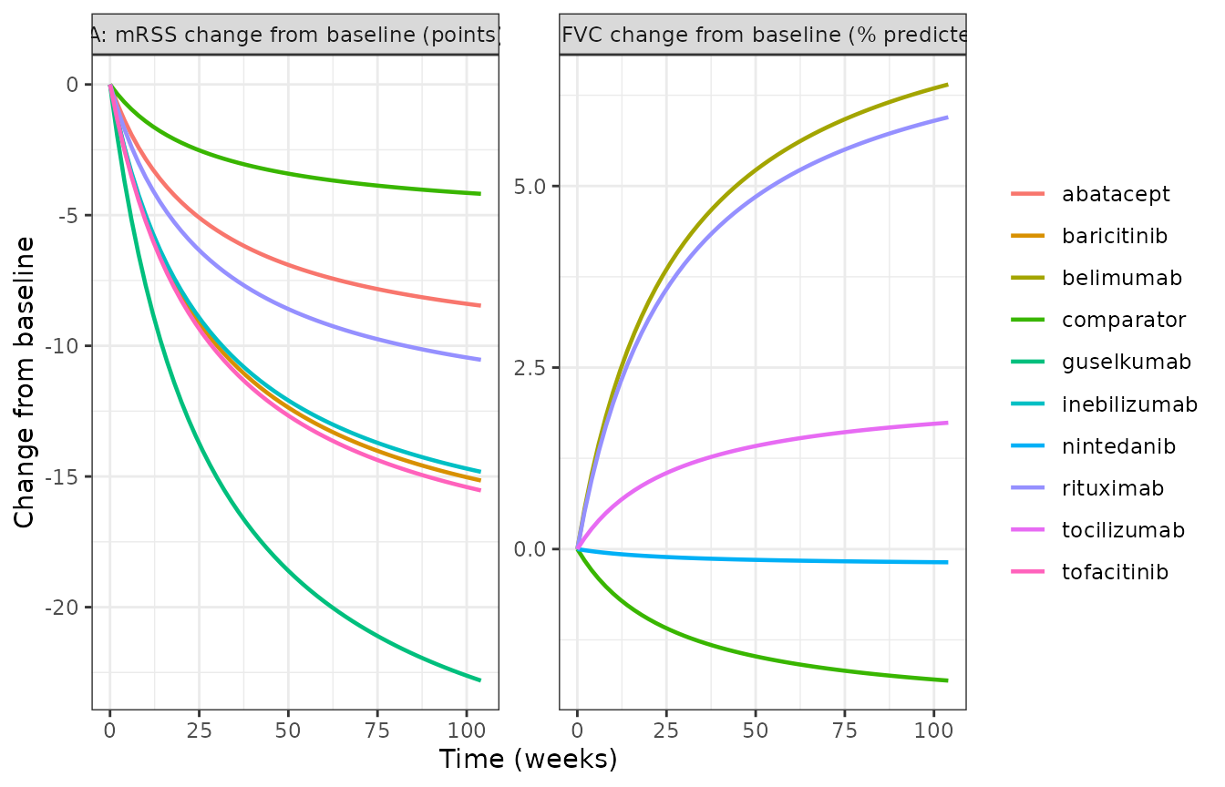
Replicates Figure 3 of Vaskeikina 2026: typical change from baseline for the comparator and each therapy with a distinguishable effect (A: mRSS; B: percent-predicted FVC).
At week 52 the typical changes are:
wk52 <- tv |>
  filter(time == 52) |>
  distinct(label, mrsscfb, fvcppcfb) |>
  arrange(mrsscfb)
wk52 |>
  rename("Arm" = label, "mRSS change (points)" = mrsscfb,
         "FVC change (% predicted)" = fvcppcfb) |>
knitr::kable(digits = 2)| Arm | mRSS change (points) | FVC change (% predicted) |
|---|---|---|
| guselkumab | -18.87 | -1.50 |
| tofacitinib | -12.85 | -1.50 |
| baricitinib | -12.53 | -1.50 |
| inebilizumab | -12.26 | -1.50 |
| rituximab | -8.71 | 4.92 |
| abatacept | -7.00 | -1.50 |
| comparator | -3.46 | -1.50 |
| belimumab | -3.46 | 5.29 |
| nintedanib | -3.46 | -0.15 |
| tocilizumab | -3.46 | 1.44 |
f52 <- 52 / (27.49 + 52)
get52 <- function(lbl, col) wk52[[col]][wk52$label == lbl]
stopifnot(
  abs(get52("comparator", "mrsscfb") - (-5.29) * f52) < 1e-8,
  abs(get52("guselkumab", "mrsscfb") - (-5.29 - 23.55) * f52) < 1e-8,
  abs(get52("rituximab", "fvcppcfb") - (-2.29 + 9.81) * f52) < 1e-8,
  # Section 3.2 ranking: guselkumab has the largest mRSS effect and belimumab
  # the largest FVC effect; rituximab is the only drug acting on both.
  wk52$label[which.min(wk52$mrsscfb)] == "guselkumab",
  wk52$label[which.max(wk52$fvcppcfb)] == "belimumab",
  get52("rituximab", "mrsscfb") < get52("comparator", "mrsscfb"),
  get52("rituximab", "fvcppcfb") > get52("comparator", "fvcppcfb")
)
Replication of Figure 4A: rituximab versus control at three arm sizes
Section 2.4 simulates rituximab and control arms of 15, 46 and 288
patients (the median, mean and maximum arm sizes in the database),
including BTAV and residual variability but not BSV (Equations 12 and
13). Here each arm size and treatment has 200 simulated arms. The model
draws the between-study term too; because it is additive on Emax it is
removed exactly afterwards by subtracting
eta_study_emax_<endpoint> * t / (ET50 + t).
rxode2::rxSetSeed(20261017)
n_rep <- 200L
arms_4a <- tidyr::expand_grid(N_ARM = c(15, 46, 288), TRT_RITUXIMAB = c(0, 1), rep = seq_len(n_rep)) |>
  mutate(id = row_number())
sim_4a <- rxode2::rxSolve(mod, make_events(arms_4a |> select(-rep), seq(0, 52, by = 2)))
prm_4a <- as.data.frame(sim_4a$params) |> mutate(id = as.integer(as.character(id)))

traj_4a <- as.data.frame(sim_4a) |>
  mutate(id = as.integer(id)) |>
  left_join(prm_4a[, c("id", "eta_study_emax_mrss", "eta_study_emax_fvc")], by = "id") |>
  mutate(
    endpoint = ifelse(CMT == 1, "mRSS (points)", "FVC (% predicted)"),
    bsv = ifelse(CMT == 1, eta_study_emax_mrss, eta_study_emax_fvc) * tcourse,
    value = sim - bsv,
    arm = ifelse(TRT_RITUXIMAB == 1, "rituximab", "control")
  )

summ_4a <- traj_4a |>
  group_by(endpoint, N_ARM, arm, time) |>
  summarise(mean = mean(value), lo = quantile(value, 0.025), hi = quantile(value, 0.975),
            .groups = "drop")

ggplot(summ_4a, aes(time, mean, colour = arm, fill = arm)) +
  geom_ribbon(aes(ymin = lo, ymax = hi), alpha = 0.2, colour = NA) +
  geom_line() +
  facet_grid(endpoint ~ paste("N =", N_ARM), scales = "free_y") +
  labs(x = "Time (weeks)", y = "Change from baseline", colour = NULL, fill = NULL) +
  theme_bw()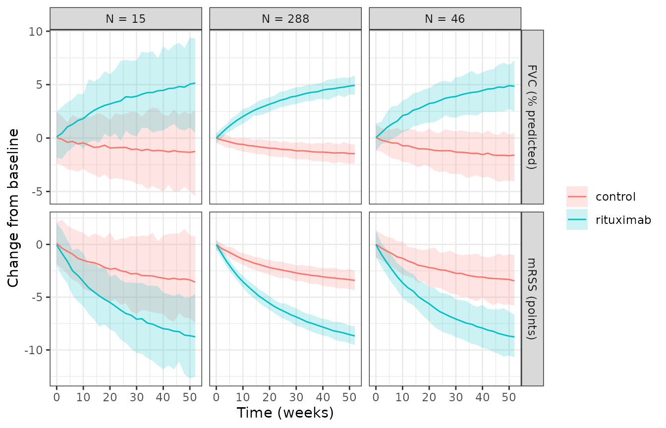
Replicates Figure 4A of Vaskeikina 2026: mean and 95% interval of simulated arm-mean change from baseline for rituximab and control arms of 15, 46 and 288 patients (BTAV and residual variability; no BSV).
The interval narrows with arm size roughly as 1/sqrt(N),
and the mean is the typical value regardless of arm size:
w52 <- summ_4a |> filter(time == 52) |> mutate(width = hi - lo)
typ52 <- function(e, a) {
  base <- if (e == "mRSS (points)") -5.29 + (a == "rituximab") * -8.03 else -2.29 + (a == "rituximab") * 9.81
  base * 52 / (27.49 + 52)
}
w52$typ <- mapply(typ52, w52$endpoint, w52$arm)
ratio <- w52 |>
  select(endpoint, arm, N_ARM, width) |>
  tidyr::pivot_wider(names_from = N_ARM, values_from = width, names_prefix = "w")
stopifnot(
  # Mean of 200 arms within a few standard errors of the typical value.
  all(abs(w52$mean - w52$typ) < 4 * (w52$hi - w52$lo) / 3.92 / sqrt(n_rep)),
  # Width ratio 15 vs 288 should be sqrt(288 / 15) = 4.38.
  all(abs(ratio$w15 / ratio$w288 / sqrt(288 / 15) - 1) < 0.3)
)
Replication of Figure 4B: time to a detectable treatment effect
Section 2.4 defines the earliest detectable time as the first week at which the 95% interval of the difference between paired simulated rituximab and control trajectories excludes zero, and Section 3.3 reports 3 weeks (N = 288) and 17 weeks (N = 15) for mRSS, and 3 to 14 weeks for FVC.
Because every term is normal, the difference at time t is
normal with mean beta * f(t)
(f(t) = t / (ET50 + t)) and a variance of
2 sigma^2 / N from the two arms’ residuals, plus
2 gamma^2 f(t)^2 / N if the two arms’ BTAV draws are
independent. The detection week is therefore available in closed form
under either reading:
et50 <- 27.49
detect_week <- function(beta, sigma, gamma, n, btav, weeks = 1:156) {
  f <- weeks / (et50 + weeks)
  sd_diff <- sqrt(2 / n * (sigma^2 + btav * gamma^2 * f^2))
  hit <- abs(beta) * f > qnorm(0.975) * sd_diff
  if (any(hit)) weeks[which(hit)[1]] else NA_integer_
}
det <- tidyr::expand_grid(
  tibble(endpoint = c("mRSS", "FVC"), beta = c(-8.03, 9.81), sigma = c(4.12, 4.42),
         gamma = c(10.23, 9.94), paper_n15 = c(17, 14), paper_n288 = c(3, 3)),
  N = c(15, 46, 288)
) |>
  rowwise() |>
  mutate(
    week_residual_only = detect_week(beta, sigma, gamma, N, btav = 0),
    week_with_btav = detect_week(beta, sigma, gamma, N, btav = 1)
  ) |>
  ungroup()

det |>
  select(endpoint, N, week_residual_only, week_with_btav) |>
  rename("Endpoint" = endpoint, "Arm size" = N,
         "Week (residual only)" = week_residual_only,
         "Week (independent BTAV)" = week_with_btav) |>
knitr::kable()| Endpoint | Arm size | Week (residual only) | Week (independent BTAV) |
|---|---|---|---|
| mRSS | 15 | 16 | NA |
| mRSS | 46 | 8 | 9 |
| mRSS | 288 | 3 | 3 |
| FVC | 15 | 14 | 25 |
| FVC | 46 | 7 | 7 |
| FVC | 288 | 3 | 3 |
# The residual-only reading reproduces every value Section 3.3 reports. The
# published detection time comes from 1000 Monte Carlo pairs, so a one-week
# difference at N = 15 is within its sampling error (the margin at week 16 is
# a fraction of a percent of the difference SD).
d15 <- det |> filter(N == 15)
d288 <- det |> filter(N == 288)
stopifnot(
  all(abs(d15$week_residual_only - d15$paper_n15) <= 1),
  all(d288$week_residual_only == d288$paper_n288)
)
The residual-only reading reproduces the published times; with independent BTAV draws, the mRSS difference at N = 15 would not be detectable within three years. So in the paper’s paired trajectories the rituximab and control arms share their between-arm deviation and differ only by the residual. The curve of Figure 4B follows from the same expression:
curve_4b <- tidyr::expand_grid(
  tibble(endpoint = c("mRSS", "FVC"), sigma = c(4.12, 4.42)),
  beta = seq(2, 25, by = 0.5),
  N = c(15, 46, 288)
) |>
  rowwise() |>
  mutate(week = detect_week(beta, sigma, 0, N, btav = 0)) |>
  ungroup() |>
  # Small effects in small arms are not detectable within three years.
  filter(!is.na(week))

ggplot(curve_4b, aes(beta, week, colour = factor(N))) +
  geom_line() +
  facet_wrap(~endpoint) +
  labs(x = "Absolute treatment effect |beta|", y = "Earliest detectable week",
       colour = "Arm size") +
  theme_bw()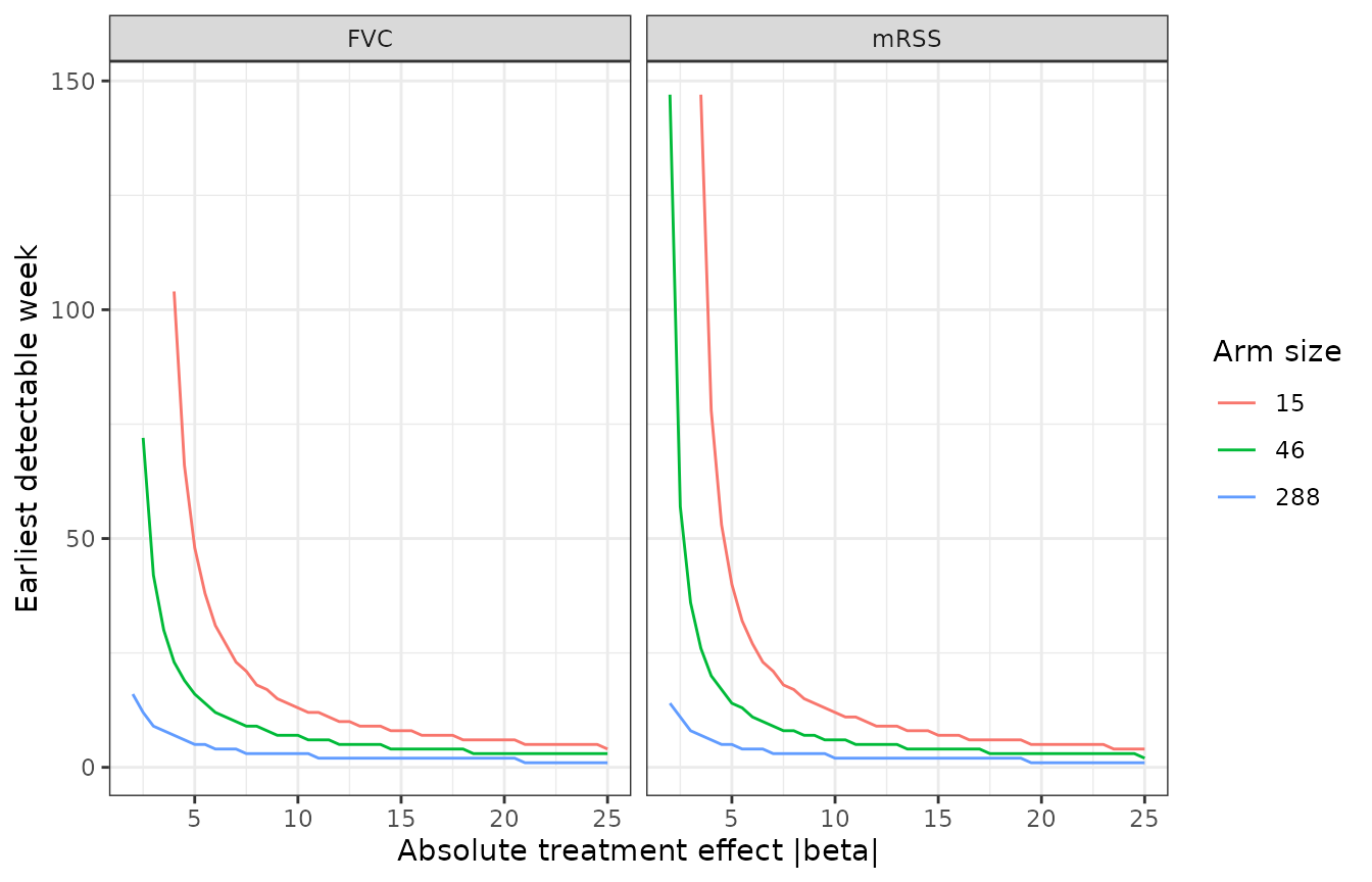
Replicates Figure 4B of Vaskeikina 2026: earliest week at which a treatment effect of size beta becomes detectable, by arm size (residual-only reading).
Assumptions and deviations
-
ET50 is stored on the log scale
(
let50 = log(27.49)) to keep it positive; the paper reports it on the linear scale with no random effect, so predictions are identical. -
Arm size is a required input.
N_ARMmust be supplied on every row; the between-arm random effect and the residual are both divided bysqrt(N_ARM)(Equations 9 and 10). The between-study random effect is not. -
Each simulated
idis one study arm, and draws its own between-study effect. To simulate several arms of one study, give them the sameeta_study_*values yourself; to reproduce the paper’s Figure 3 and 4 scenarios, remove the between-study term as done above. - Paired trajectories in Figure 4B. Section 2.4 does not say whether the paired rituximab and control trajectories share their BTAV draw. Only the shared (residual-only) reading reproduces the detection times of Section 3.3, as shown above.
- Drugs without a retained effect are not in the model. Fourteen agents for mRSS and sixteen for FVC (Section 3.2) had effects that could not be distinguished from the comparator; agents whose effect had an RSE above 50% were removed from the fit, keeping their control arms (Section 2.3.2). Setting every indicator to 0 for such a drug predicts the comparator response, which is not a claim the paper makes.
- Parameter uncertainty is not reproduced. The paper’s Figure 3 intervals sample the estimates’ variance-covariance matrix, which is not published; the RSEs in Table 1 alone do not determine it.
- The supplement (search strategy, per-trial characteristics and diagnostic plots) was not used; every value and equation the model needs is in the main article.
Errata
- Section 3.2 and the Abstract describe inebilizumab as an “anti-BAFF antibody”; it is an anti-CD19 antibody (belimumab is the anti-BAFF agent). Section 3.2 also calls abatacept an “anti-CTLA-4 antibody”; it is a CTLA-4-Ig fusion protein. Neither affects a parameter.
- The Abstract and Section 3.2 list inebilizumab before baricitinib in the mRSS ranking, but Table 1 gives baricitinib the slightly larger effect (-13.87 versus -13.45 points). The model uses the Table 1 values.
- Section 2.4 gives the mean arm size as 45 and Section 3.3 and the Figure 4 caption as 46; 46 is used here.