Endotoxin, TNF-alpha and IL-6 in piglets (Thorsted 2019) • nlmixr2lib

Model and source

mod <- readModelDb("Thorsted_2019_endotoxin")
ui <- rxode2::rxode(mod)
#> ℹ parameter labels from comments will be replaced by 'label()'

Citation: Thorsted A, Bouchene S, Tano E, Castegren M, Lipcsey M, Sjolin J, Karlsson MO, Friberg LE, Nielsen EI. (2019). A non-linear mixed effect model for innate immune response: In vivo kinetics of endotoxin and its induction of the cytokines tumor necrosis factor alpha and interleukin-6. PLoS ONE 14(2):e0211981. doi:10.1371/journal.pone.0211981.
Description: Preclinical (piglet). Semi-mechanistic model of intravenously infused E. coli O111:B4 endotoxin (ETX) and the innate cytokine response it induces in anaesthetised piglets (Thorsted 2019). ETX follows one-compartment disposition with Michaelis-Menten elimination plus a constant assay baseline. ETX stimulates TNF-alpha production through a sigmoidal Emax whose EC50 is itself raised by ETX through a three-stage moderator chain (endotoxin tolerance). IL-6 production is stimulated linearly by the relative increase in TNF-alpha and by ETX, with appearance in plasma delayed by four transit compartments. A mixture sub-population (MIX_ETX_CONTAM) carries pre-study contaminating ETX that is measured but does not drive the cytokines, so the model keeps a second, identically eliminated ETX pool (central_contam) for the assay read-out. Every infusion must be given to both central and central_contam.
Article: https://doi.org/10.1371/journal.pone.0211981 (PMC6383944, open access)
Supplements: S1 Text (the final NONMEM control stream, with every ODE) and S1 Table (the 116-piglet modelling dataset), both deposited with the PLOS ONE record.

Thorsted 2019 is a semi-mechanistic model of the innate immune response to intravenously infused endotoxin (ETX, E. coli O111:B4) in anaesthetised piglets. It links three measured time-courses:

ETX follows one-compartment disposition with Michaelis-Menten elimination and a constant assay baseline.
TNF-alpha follows a turnover model whose production rate is stimulated by a sigmoidal Emax in the ETX concentration.
IL-6 follows a turnover model whose production rate is stimulated linearly by the relative increase in TNF-alpha and by ETX, with plasma appearance delayed through four transit compartments.

Endotoxin tolerance is built in: the ETX concentration raises EC50 of the ETX-TNF-alpha relationship through a three-stage moderator chain, so continued exposure progressively blunts the TNF-alpha response.

Why two endotoxin compartments

The source $MODEL block declares two ETX compartments with identical kinetics (same Vmax, KM, Vc) that receive the same infusion and differ only in their initial condition:

central starts at zero. Only this pool drives TNF-alpha and IL-6, because (Results, “Host response”) control groups showed no cytokine response to the constant baseline or to the pre-study contamination.
central_contam starts at a pre-study contaminating amount in the contamination mixture sub-population (MIX_ETX_CONTAM = 1, Eq 1). The measured endotoxin concentration is Cc = rbase_etx + central_contam / vc.

Because elimination is Michaelis-Menten, the two pools are not additively separable, so a single state cannot give both the measured concentration and the pharmacologically active one. Every dosing record must therefore be given to both compartments; the source dataset does this with two EVID = 1 rows (CMT 1 and CMT 2) of the same amount and rate.

This is an endogenous / mechanistic model: there is no classical absorption-distribution-elimination profile of an administered drug to integrate (the “drug” is an immune stimulus), so NCA is not the right validation. Instead the sections below check the biological steady state, recovery after a perturbation, mass balance at steady state, dimensional consistency, and reproduction of the paper’s Figure 6.

Population

The model was fit to 116 anaesthetised piglets (approximately 12 weeks old, mean weight approximately 27 kg) pooled across six studies (A-F; Thorsted 2019 Table 1), contributing 278 ETX, 1068 TNF-alpha and 1045 IL-6 observations. ETX was infused intravenously for 1-30 h at 0 (saline) to 16.0 ug/kg/h; the batch potency was 1000 EU/ug (studies A, B, E) or 3000 EU/ug (studies C, D, F). ETX was measured in studies C, E and F only. A seventh study (G, n = 6) was held out for external evaluation and is not part of the fit.

mod()$population
#> $species
#> [1] "pig (anaesthetised piglets)"
#> 
#> $n_subjects
#> [1] 116
#> 
#> $n_studies
#> [1] 6
#> 
#> $age_range
#> [1] "approximately 12 weeks"
#> 
#> $weight_median
#> [1] "mean approximately 27 kg"
#> 
#> $disease_state
#> [1] "experimental endotoxaemia (porcine endotoxin model); saline-infused controls included"
#> 
#> $dose_range
#> [1] "Continuous IV infusion of E. coli O111:B4 endotoxin for 1-30 h at 0 (saline) to 16.0 ug/kg/h; batch potency 1000 EU/ug (studies A, B, E) or 3000 EU/ug (studies C, D, F)"
#> 
#> $regions
#> [1] "Sweden (Uppsala University Hospital)"
#> 
#> $notes
#> [1] "Six studies (A-F, Thorsted 2019 Table 1) pooled: 278 ETX, 1068 TNF-alpha and 1045 IL-6 observations. ETX was measured in studies C, E and F only. A seventh study (G, n = 6) was held out for external evaluation and is not part of the fit. Sex not reported."

Source trace

Every ini() value is traced to its source in an in-file comment next to the parameter in inst/modeldb/pharmacodynamics/Thorsted_2019_endotoxin.R. The table collects them. Structure is from S1 Text; final values are from Table 2 (the stream’s $THETA/$OMEGA blocks are the run045 initial estimates, e.g. KM 12325.3 vs Table 2’s 12600, so Table 2 governs per the standard initial-vs-final rule).

Parameter	Value	Source
`lvmax`	442000 EU/h	Table 2 `Vmax`
`lkm`	12600 EU/L	Table 2 `KM`
`lvc`	36.1 L	Table 2 `Vc`
`lrbase_etx` / `lrbase_etx_f`	155 / 1810 EU/L	Table 2 `BASE ETX` (Endochrome C+E / Coatest F)
`lprop_cont`	132	Table 2 `Propcont`; Eq 1
`lmtt_tnf`	1.04 h	Table 2 `MTT TNF-alpha`
`lrbase_tnf` / `_e` / `_cf` / `_d`	281 / 25.4 / 3.06 / 68.2 ng/L	Table 2 `S0,TNF-alpha` (DuoSet A+B / DuoSet E / BioSource C+F / BioSource D)
`lemax_tnf`	2540	Table 2 `Emax`
`lec50_tnf`	286 EU/L	Table 2 `EC0`
`lhill_tnf`	2.10	Table 2 `gamma`
`lmtt_tol`	6.33 h	Table 2 `MTT EC50`
`lemax_tol`	45100	Table 2 `Tmax`
`lec50_tol`	29300 EU/L	Table 2 `TC50`
`lmtt_il6`	1.45 h	Table 2 `MTT IL-6`
`lrbase_il6` / `_cdf`	49.2 / 8.19 ng/L	Table 2 `S0,IL-6` (DuoSet A+B+E / BioSource C+D+F)
`lslope_tnf`	0.961	Table 2 `ESLP,TNF-alpha`; Eq 2
`lslope_etx`	0.00937	Table 2 `ESLP,ETX`
`expSd` / `expSd_tnf` / `expSd_il6`	0.321 / 0.485 / 0.505	Table 2 residual error
IIV (6 terms + KM-Vc correlation)	see below	Table 2 CV%; r(KM,Vc) = -0.42
`d/dt(central)`, `d/dt(central_contam)`	n/a	S1 Text `$DES` (Michaelis-Menten ETX)
`d/dt(tnf)`	n/a	S1 Text `$DES`; Eq 3
`d/dt(moderator1..3)`	n/a	S1 Text `$DES` (tolerance chain)
`d/dt(transit1..4)`, `d/dt(il6)`	n/a	S1 Text `$DES`; Eq 2

IIV reading. Table 2 footnote c reports variability “on the approximate standard deviation scale”, and 100 * sqrt(omega^2) reproduces the printed CV% column against the stream’s $OMEGA variances (e.g. KM: 100*sqrt(1.44) = 120, matching the printed 120; the exact log-normal CV would be 180). So the variances are omega^2 = (CV/100)^2, and the KM-Vc covariance is -0.42 * 1.20 * 0.753 = -0.3795 (Results reports the correlation as -0.42; the stream’s block gives -0.4251).

Units table (dimensional check)

ODE term	Units multiply to	Equals `d/dt(state)`
`vmax * (A/vc) / (km + A/vc)`	(EU/h)(EU/L)/(EU/L) = EU/h	EU/h
`kin_tnf * (1 + eff_tnf)`	(ng/L / h)(unitless) = ng/L/h	ng/L/h
`kout_tnf * tnf`	(1/h)(ng/L) = ng/L/h	ng/L/h
`kin_tol * (1 + tol)`	(EU/L / h)(unitless) = EU/L/h	EU/L/h
`kout_il6 * transit`	(1/h)(ng/L) = ng/L/h	ng/L/h
`slope_etx * cp_etx`	(L/EU)(EU/L) = unitless	n/a (adds to stimulation)

eff_il6 = slope_tnf * (tnf/rbase_tnf - 1) + slope_etx * cp_etx is unitless, as required of a multiplier on the IL-6 production rate: the TNF-alpha term is a ratio and slope_etx carries L/EU to cancel the EU/L of cp_etx.

Steady-state check

With no infusion the system must sit at its biological baseline indefinitely: measured ETX at rbase_etx, TNF-alpha at rbase_tnf, IL-6 at rbase_il6, and EC50 at EC0. Solve the typical-value model (study A/B, no contamination) for 60 h with no dose.

typ <- mod |> rxode2::zeroRe()
#> ℹ parameter labels from comments will be replaced by 'label()'

cov0 <- list(
  MIX_ETX_CONTAM = 0, STUDY_ETX_C = 0, STUDY_ETX_D = 0,
  STUDY_ETX_E = 0, STUDY_ETX_F = 0
)

# The model has three endpoints (Cc, tnf, il6), so rxode2 only accepts an
# observation row whose `cmt` is one of them. `tnf` is both an endpoint and an
# ODE state, so it is used throughout; rxode2 still returns every state and Cc
# on each row.
obs_rows <- function(times, covs) {
  out <- data.frame(id = 1L, time = times, evid = 0L, amt = 0, cmt = "tnf")
  for (nm in names(covs)) out[[nm]] <- covs[[nm]]
  out
}

ev_ss <- obs_rows(seq(0, 60, by = 1), cov0)

s_ss <- rxode2::rxSolve(typ, ev_ss, returnType = "data.frame")
#> ℹ omega/sigma items treated as zero: 'etalkm', 'etalvc', 'etalrbase_etx', 'etalmtt_tnf', 'etalrbase_tnf', 'etalmtt_il6', 'etalrbase_il6'

# ETX, TNF-alpha, IL-6 and EC50 should hold at the reported baselines.
stopifnot(
  max(abs(s_ss$Cc - 155)) < 1e-6,
  max(abs(s_ss$tnf - 281)) < 1e-4,
  max(abs(s_ss$il6 - 49.2)) < 1e-4,
  max(abs(s_ss$moderator3 - 286)) < 1e-4
)
range(s_ss$tnf)
#> [1] 281 281
range(s_ss$il6)
#> [1] 49.2 49.2

In the contamination sub-population the measured ETX must start at the assay baseline plus the contaminating amount of Eq 1:

cov_c <- cov0
cov_c$MIX_ETX_CONTAM <- 1
ev_c <- obs_rows(seq(0, 6, by = 0.5), cov_c)

s_c <- rxode2::rxSolve(typ, ev_c, returnType = "data.frame")
#> ℹ omega/sigma items treated as zero: 'etalkm', 'etalvc', 'etalrbase_etx', 'etalmtt_tnf', 'etalrbase_tnf', 'etalmtt_il6', 'etalrbase_il6'
# central_contam(0) = rbase_etx * prop_cont = 155 * 132 = 20460 EU;
# Cc(0) = rbase_etx + 20460/vc = 155 + 20460/36.1.
stopifnot(abs(s_c$Cc[s_c$time == 0] - (155 + 155 * 132 / 36.1)) < 1e-6)
s_c$Cc[s_c$time == 0]
#> [1] 721.759

Perturbation recovery

rxSolve(inits = ) cannot be used to displace the cytokines, because the model sets tnf(0) and il6(0) from their baselines and that assignment takes precedence. Two perturbations are applied with events instead, and each is first asserted to have moved the system before its recovery is checked:

a bolus that doubles TNF-alpha and IL-6 at t = 0 with no ETX present;
a 1 h ETX infusion at 4000 EU/kg/h (27 kg piglet) into both ETX pools, which stimulates both cytokines and raises EC50 through the tolerance chain.

After the ETX has been eliminated, every state must return to its baseline.

obs_grid <- seq(0, 72, by = 0.5)

ev_bolus <- dplyr::bind_rows(
  data.frame(id = 1L, time = 0, evid = 1L, amt = c(281, 49.2),
             cmt = c("tnf", "il6")),
  obs_rows(obs_grid, list())
)
for (nm in names(cov0)) ev_bolus[[nm]] <- cov0[[nm]]

pulse_rate <- 4000 * 27 # EU/h
ev_pulse <- dplyr::bind_rows(
  data.frame(id = 1L, time = 0, evid = 1L, amt = pulse_rate, rate = pulse_rate,
             cmt = c("central", "central_contam")),
  obs_rows(obs_grid, list())
)
for (nm in names(cov0)) ev_pulse[[nm]] <- cov0[[nm]]

s_bolus <- rxode2::rxSolve(typ, ev_bolus, returnType = "data.frame")
#> ℹ omega/sigma items treated as zero: 'etalkm', 'etalvc', 'etalrbase_etx', 'etalmtt_tnf', 'etalrbase_tnf', 'etalmtt_il6', 'etalrbase_il6'
s_pulse <- rxode2::rxSolve(typ, ev_pulse, returnType = "data.frame")
#> ℹ omega/sigma items treated as zero: 'etalkm', 'etalvc', 'etalrbase_etx', 'etalmtt_tnf', 'etalrbase_tnf', 'etalmtt_il6', 'etalrbase_il6'

end_of <- function(s) s[s$time == max(s$time), ]
rel_dev <- function(x, ref) abs(x / ref - 1)

stopifnot(
  # The perturbations happened.
  max(s_bolus$tnf) > 1.5 * 281,
  max(s_bolus$il6) > 1.5 * 49.2,
  max(s_pulse$tnf) > 10 * 281,
  max(s_pulse$il6) > 10 * 49.2,
  max(s_pulse$moderator3) > 10 * 286,
  # ...and every state relaxed back to its baseline by 72 h.
  rel_dev(end_of(s_bolus)$tnf, 281) < 0.01,
  rel_dev(end_of(s_bolus)$il6, 49.2) < 0.01,
  rel_dev(end_of(s_pulse)$tnf, 281) < 0.01,
  rel_dev(end_of(s_pulse)$il6, 49.2) < 0.01,
  rel_dev(end_of(s_pulse)$moderator3, 286) < 0.01,
  rel_dev(end_of(s_pulse)$Cc, 155) < 0.01
)

dplyr::bind_rows(
  transform(s_bolus, perturbation = "Cytokine bolus (2x baseline)"),
  transform(s_pulse, perturbation = "1 h ETX pulse, 4000 EU/kg/h")
) |>
  dplyr::select(time, perturbation, tnf, il6, moderator3) |>
  tidyr::pivot_longer(c(tnf, il6, moderator3), names_to = "state",
                      values_to = "value") |>
  ggplot(aes(time, value, colour = perturbation)) +
  geom_line() +
  facet_wrap(~state, scales = "free_y") +
  scale_y_log10() +
  labs(x = "Time (h)", y = "Value (ng/L; EC50 in EU/L)",
       title = "Perturbation recovery to baseline", colour = NULL) +
  theme(legend.position = "bottom")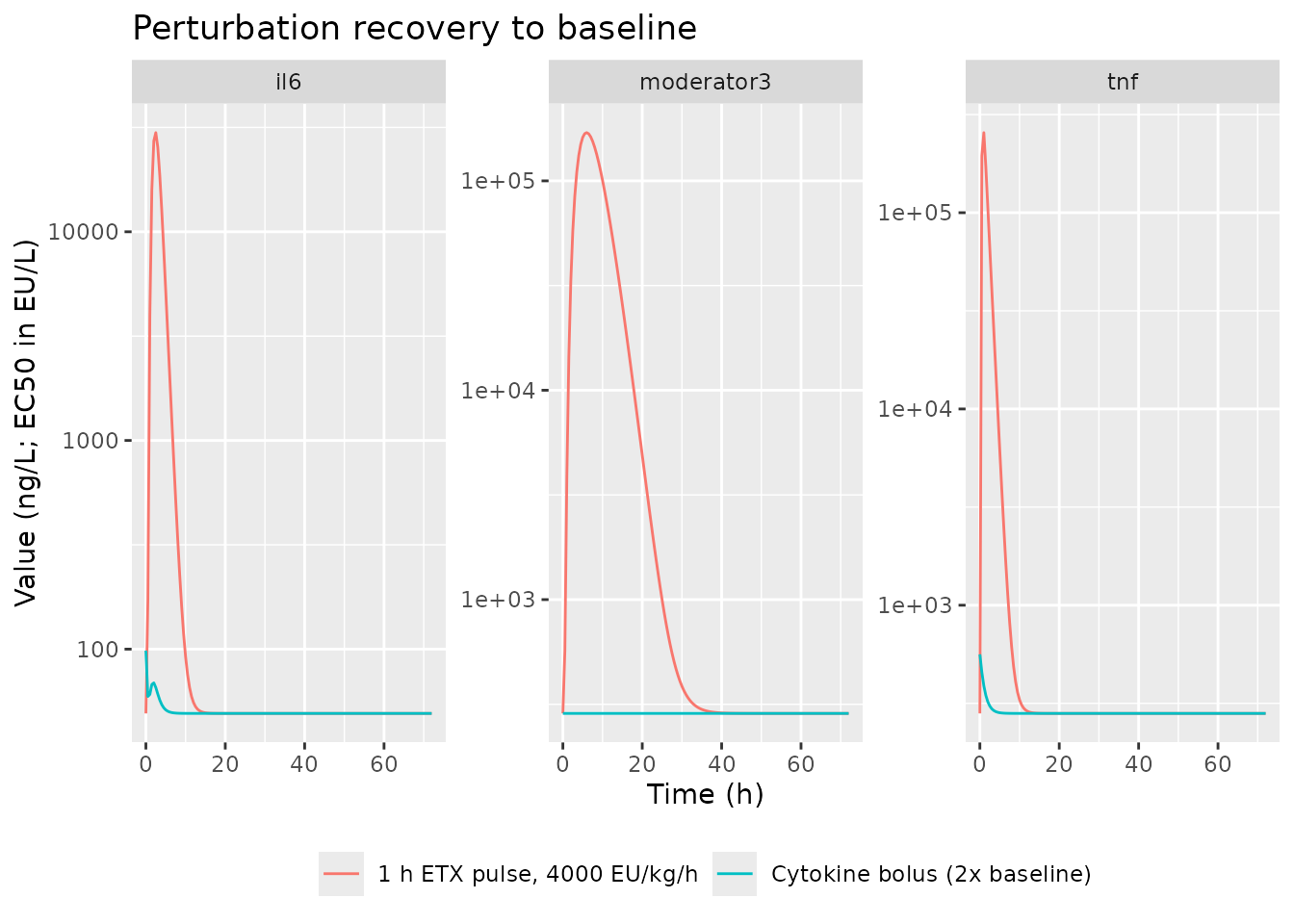

Mass-balance / flux check

At the undisturbed baseline every turnover state has production equal to elimination, so d/dt = 0. Verify symbolically for TNF-alpha and IL-6 using the typical values.

rbase_tnf <- 281; mtt_tnf <- 1.04
kout_tnf <- 1 / mtt_tnf
kin_tnf <- rbase_tnf * kout_tnf
# With no ETX: eff_tnf = 0, so d/dt(tnf) = kin_tnf - kout_tnf * rbase_tnf.
stopifnot(abs(kin_tnf - kout_tnf * rbase_tnf) < 1e-9)

rbase_il6 <- 49.2; mtt_il6 <- 1.45
kout_il6 <- 5 / mtt_il6
kin_il6 <- rbase_il6 * kout_il6
# Each IL-6 chain stage flows at kout_il6 * rbase_il6 in and out at baseline.
stopifnot(abs(kin_il6 - kout_il6 * rbase_il6) < 1e-9)

# EC50 chain: kin_tol = EC0 * kout_tol, so the chain holds at EC0 with no ETX.
ec0 <- 286; mtt_tol <- 6.33
kout_tol <- 3 / mtt_tol
kin_tol <- ec0 * kout_tol
stopifnot(abs(kin_tol - kout_tol * ec0) < 1e-9)
c(kin_tnf = kin_tnf, kin_il6 = kin_il6, kin_tol = kin_tol)
#>  kin_tnf  kin_il6  kin_tol 
#> 270.1923 169.6552 135.5450

Replicate Figure 6

Figure 6 shows typical-value 30 h predictions of ETX (A), TNF-alpha (B), IL-6 (C) and the potency parameter EC50 (D) across initial infusion rates of 63, 250, 500, 1000, 4000, 8000 and 16000 EU/kg/h, with the four lowest rates switched to 4000 EU/kg/h after 15 h to demonstrate tolerance (an infusion dataset uses EU, so the per-kg rate times the 27 kg mean weight gives the EU/h infusion). The model has no weight covariate; the per-kg scaling is applied when the event table is built. Each infusion goes to both ETX compartments.

wt <- 27 # mean piglet weight (kg), Thorsted 2019 Methods
rates <- c(63, 250, 500, 1000, 4000, 8000, 16000)

make_subject <- function(i, r) {
  switched <- r < 4000
  seg <- if (switched) {
    data.frame(time = c(0, 15), rate = c(r, 4000) * wt, dur = c(15, 15))
  } else {
    data.frame(time = 0, rate = r * wt, dur = 30)
  }
  seg$amt <- seg$rate * seg$dur
  dose <- dplyr::bind_rows(
    transform(seg, cmt = "central"),
    transform(seg, cmt = "central_contam")
  )
  dose <- dose[, c("time", "amt", "rate", "cmt")]
  dose$evid <- 1L
  obs <- data.frame(time = seq(0, 30, by = 0.25), amt = 0, rate = 0,
                    cmt = "tnf", evid = 0L)
  out <- dplyr::bind_rows(dose, obs)
  out$id <- i
  out$rate_lab <- r
  out[order(out$time, -out$evid), ]
}

ev6 <- dplyr::bind_rows(Map(make_subject, seq_along(rates), rates))
for (nm in names(cov0)) ev6[[nm]] <- cov0[[nm]]
stopifnot(!anyDuplicated(unique(ev6[, c("id", "time", "evid")])))

sim6 <- rxode2::rxSolve(typ, ev6, keep = "rate_lab",
                        returnType = "data.frame") |>
  dplyr::mutate(rate_lab = factor(rate_lab, levels = rates))
#> ℹ omega/sigma items treated as zero: 'etalkm', 'etalvc', 'etalrbase_etx', 'etalmtt_tnf', 'etalrbase_tnf', 'etalmtt_il6', 'etalrbase_il6'
#> Warning: multi-subject simulation without without 'omega'

sim6 |>
  dplyr::transmute(time, rate_lab,
                   `A: ETX (EU/L)` = Cc,
                   `B: TNF-alpha (ng/L)` = tnf,
                   `C: IL-6 (ng/L)` = il6,
                   `D: EC50 (EU/L)` = moderator3) |>
  tidyr::pivot_longer(-c(time, rate_lab), names_to = "panel",
                      values_to = "value") |>
  dplyr::filter(value > 0) |>
  ggplot(aes(time, value, colour = rate_lab)) +
  geom_line() +
  facet_wrap(~panel, scales = "free_y") +
  scale_y_log10() +
  labs(x = "Time (h)", y = NULL, colour = "Initial rate\n(EU/kg/h)",
       title = "Figure 6 - typical-value 30 h predictions",
       caption = "Replicates Figure 6 of Thorsted 2019.")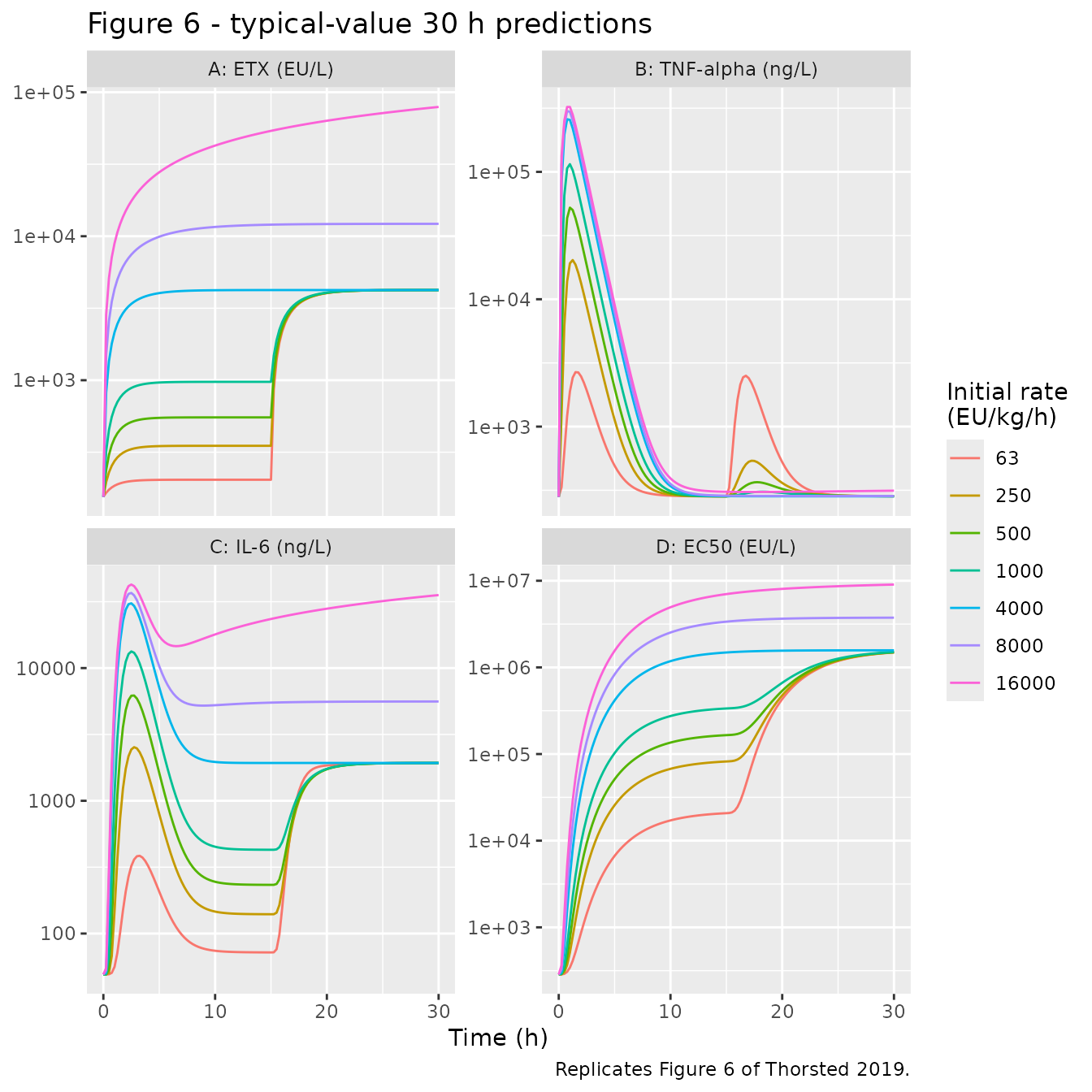

The simulation reproduces the paper’s Figure 6 behaviour:

summ <- sim6 |>
  dplyr::group_by(rate_lab) |>
  dplyr::summarise(
    etx_plateau = Cc[time == 6],
    tnf_peak = max(tnf),
    tnf_tpeak = time[which.max(tnf)],
    tnf_second = max(tnf[time > 15]),
    il6_peak = max(il6),
    ec50_end = moderator3[time == 30],
    .groups = "drop"
  )
summ
#> # A tibble: 7 × 7
#>   rate_lab etx_plateau tnf_peak tnf_tpeak tnf_second il6_peak ec50_end
#>   <fct>          <dbl>    <dbl>     <dbl>      <dbl>    <dbl>    <dbl>
#> 1 63              204.    2676.      1.5       2508.    1927. 1487817.
#> 2 250             350.   20302.      1.25       539.    2535. 1490979.
#> 3 500             550.   52373.      1          366.    6210. 1495319.
#> 4 1000            970.  114978.      1          309.   13341. 1504417.
#> 5 4000           4114.  259039.      0.75       284.   30735. 1574569.
#> 6 8000          10472.  300317.      0.75       287.   36793. 3749216.
#> 7 16000         31219.  323425.      1          314.   42569. 9039660.

stopifnot(
  # ETX plateau rises monotonically with infusion rate (Panel A).
  all(diff(summ$etx_plateau) > 0),
  # TNF-alpha peaks within the first few hours (Panel B).
  all(summ$tnf_tpeak <= 3),
  # TNF-alpha response increases with dose (Panel B).
  all(diff(summ$tnf_peak) > 0),
  # Tolerance (Discussion, on Fig 3A): a 4000 EU/kg/h challenge after
  # pre-exposure gives a response "much lower than without any pre-exposure",
  # and lower after the higher pre-exposure. Typical values, so deterministic.
  summ$tnf_second[summ$rate_lab == "63"] < 0.05 * summ$tnf_peak[summ$rate_lab == "4000"],
  summ$tnf_second[summ$rate_lab == "250"] < summ$tnf_second[summ$rate_lab == "63"],
  # EC50 climbs far above its EC0 = 286 baseline (tolerance; Panel D).
  all(summ$ec50_end > 1e4)
)

At a constant infusion rate R (EU/h) below Vmax, Michaelis-Menten elimination has the closed-form steady state C = KM * R / (Vmax - R), and the tolerance chain then settles at EC50 = EC0 * (1 + Tmax * C / (TC50 + C)). The 4000 EU/kg/h arm (108000 EU/h) is effectively at steady state by 30 h, so its simulated ETX and EC50 must match these values. A mis-transcribed Vmax, KM, Vc, EC0, Tmax or TC50 moves them by far more than the bound.

r_4000 <- 4000 * 27
c_ss <- 12600 * r_4000 / (442000 - r_4000)
ec50_ss <- 286 * (1 + 45100 * c_ss / (29300 + c_ss))
at30 <- sim6[sim6$rate_lab == "4000" & sim6$time == 30, ]
cf <- data.frame(
  quantity = c("ETX incl. baseline (EU/L)", "EC50 (EU/L)"),
  closed_form = c(155 + c_ss, ec50_ss),
  simulated = c(at30$Cc, at30$moderator3)
)
cf$rel_diff <- cf$simulated / cf$closed_form - 1
knitr::kable(cf, digits = c(0, 1, 1, 5),
             caption = "4000 EU/kg/h arm at 30 h vs. analytic steady state.")

4000 EU/kg/h arm at 30 h vs. analytic steady state.
quantity	closed_form	simulated	rel_diff
ETX incl. baseline (EU/L)	4229.3	4229.3	0.00000
EC50 (EU/L)	1574917.3	1574568.8	-0.00022

# Measured residuals ~2e-4 (the chains are still converging); bound 10x above.
stopifnot(all(abs(cf$rel_diff) < 2e-3))

Reading Figure 6 by eye gives the same magnitudes: ETX plateaus near 4 x 10^3 EU/L at 4000 EU/kg/h and near 8 x 10^4 EU/L at 30 h for 16000 EU/kg/h (panel A); TNF-alpha peaks near 2 x 10^3 ng/L at 63 EU/kg/h and 2.4 x 10^5 ng/L at 16000 EU/kg/h (panel B); IL-6 settles near 2 x 10^3 ng/L under 4000 EU/kg/h (panel C); and EC50 reaches about 1.5 x 10^6 EU/L at 4000 EU/kg/h and 9 x 10^6 EU/L at 16000 EU/kg/h (panel D). The figure’s control baselines sit at about 205 ng/L (TNF-alpha) and 49 ng/L (IL-6), the EBE-median DuoSet baselines the paper used for study G, rather than the study A/B typical values used here (281 and 49.2 ng/L). TNF-alpha production scales with its baseline, so the TNF-alpha curves here sit about 1.4-fold (281/205) above the figure’s; solving with lrbase_tnf = log(205) and lrbase_il6 = log(49.3) reproduces the figure’s levels.

Assumptions and deviations

Structure from the control stream, values from Table 2. The S1 Text $THETA/$OMEGA blocks hold the run045 initial estimates seeding the final importance-sampling run; the maintainers took every final value from Table 2, following the standard rule that a results table supersedes control-stream initials.
IIV variances read on the SD scale. Table 2 reports variability as a CV% that equals 100 * sqrt(omega^2) (footnote c, “approximate standard deviation scale”), so the variances encoded are (CV/100)^2 and the KM-Vc covariance is -0.42 * 1.20 * 0.753 = -0.3795. The six fixed $OMEGA variances (0.000625) in the stream are structural parameters the paper did not vary and carry no IIV in the model.
Residual error is additive on log-transformed data, which the maintainers encoded as lnorm() (Methods, “an additive relation was used for RUV (approximately proportional with log-transformed data)”); the BLOQ M3 likelihood handling in the stream is an estimation detail with no bearing on simulation.
The mixture probability (0.399, fixed) is not an ini() parameter. Following the MIX_LARGE_BASE precedent, it is documented in the MIX_ETX_CONTAM covariate entry; set the covariate to 0 for a typical uncontaminated animal or draw Bernoulli(0.399) per subject for a population.
No weight covariate. The model reads no body weight; infusion rates are supplied in EU/h, so the per-kg rates of Figure 6 are multiplied by the 27 kg mean weight when the event table is built. Study G (external evaluation) is not part of the fit.
External-evaluation baselines. For reproducing the held-out study G (Figure 5) the paper uses EBE-median baselines of 205 ng/L (TNF-alpha) and 49.3 ng/L (IL-6); those are evaluation inputs, not model parameters, and are not encoded here.
No correction notice was found for doi:10.1371/journal.pone.0211981 as of 2026-10-16.