Relapsed/refractory multiple myeloma response-rate to PFS MBMA (Teng 2018)
Source:vignettes/articles/Teng_2018_rrmm_pfs_mbma.Rmd
Teng_2018_rrmm_pfs_mbma.RmdModel and source
- Citation: Teng Z, Gupta N, Hua Z, Liu G, Samnotra V, Venkatakrishnan K, Labotka R. Model-Based Meta-Analysis for Multiple Myeloma: A Quantitative Drug-Independent Framework for Efficient Decisions in Oncology Drug Development. Clin Transl Sci. 2018;11(3):218-225. doi:10.1111/cts.12524. Regression: Results ‘Relationship between response rates and PFS’ and Figure 1a. Data: Table 1. PTS framework: Methods ‘MBMA’ steps 1-3 and Figure 2.
- Article (open access): https://doi.org/10.1111/cts.12524
Teng 2018 is a drug-independent model-based meta-analysis (MBMA) built at Millennium (Takeda) to answer a development question: if a phase II study of a new regimen in relapsed/refractory multiple myeloma (RRMM) has reported its response rate but its progression-free survival (PFS) is still immature, how likely is a phase III trial to reach its PFS target?
The paper fits two independent linear regressions of an arm’s median PFS on its response rate, across the arms of seven phase III trials, and the library ships each as its own model:
| Model | Predictor | Published regression | R^2 |
|---|---|---|---|
Teng_2018_rrmm_pfs_orr_mbma |
overall response rate, ORR = CR + VGPR + PR (%) | mPFS = -23.46 + 0.56 * ORR | 0.84 |
Teng_2018_rrmm_pfs_vgpr_mbma |
very good partial response or better, >=VGPR = CR + VGPR (%) | mPFS = 2.62 + 0.34 * >=VGPR | 0.75 |
Every observation is a trial arm, not a patient. There is no dose, no exposure and no time course; each arm contributes one response rate and one median PFS. Non-compartmental analysis therefore does not apply, and validation here is against the paper’s own data table and its own worked numbers.
mod_orr <- readModelDb("Teng_2018_rrmm_pfs_orr_mbma")
mod_vgpr <- readModelDb("Teng_2018_rrmm_pfs_vgpr_mbma")
ui_orr <- rxode2::rxode(mod_orr)
ui_vgpr <- rxode2::rxode(mod_vgpr)
Population
Seven randomised controlled phase III trials in RRMM that reported PFS between 2014 and 2017, identified from the van Beurden-Tan 2017 systematic review, covering 4,924 patients who had received at least one prior line of therapy (primarily one to three). The investigational regimens span proteasome inhibitors (ixazomib, carfilzomib), an HDAC inhibitor (panobinostat), an anti-SLAMF7 antibody (elotuzumab) and an anti-CD38 antibody (daratumumab), on lenalidomide-dexamethasone (Rd) or bortezomib-dexamethasone (Vd) backbones. Table 1 of the paper lists all 14 arms; the two daratumumab arms are excluded from the fit because their median PFS had not been reached, leaving 12 arms.
table1 <- data.frame(
  study = c(
    "TOURMALINE-MM1", "TOURMALINE-MM1", "ASPIRE", "ASPIRE",
    "ENDEAVOR", "ENDEAVOR", "PANORAMA-1", "PANORAMA-1",
    "ELOQUENT-2", "ELOQUENT-2", "POLLUX", "POLLUX", "CASTOR", "CASTOR"
  ),
  arm = c(
    "Ixazomib-Rd", "Placebo-Rd", "Carfilzomib-Rd", "Rd",
    "Carfilzomib-dexamethasone", "Vd", "Panobinostat-Vd", "Placebo-Vd",
    "Elotuzumab-Rd", "Rd", "Daratumumab-Rd", "Rd", "Daratumumab-Vd", "Vd"
  ),
  n = c(360, 362, 396, 396, 464, 465, 387, 381, 321, 325, 286, 283, 251, 247),
  orr = c(78, 72, 87.1, 66.7, 77, 63, 60.7, 54.6, 79, 66, 93, 76, 82.9, 63.2),
  vgpr = c(48, 39, 69.9, 40.4, 54, 29, 27.6, 15.7, 33, 28, 74, 44, 59.2, 29.1),
  pfs = c(20.6, 14.7, 26.3, 17.6, 18.7, 9.4, 11.99, 8.08, 19.4, 14.9, NA, 18.4, NA, 7.2)
)
fitset <- dplyr::filter(table1, !is.na(pfs))

table1 |>
  dplyr::rename(
    "Study" = study, "Arm" = arm, "N" = n, "ORR (%)" = orr,
    ">=VGPR (%)" = vgpr, "Median PFS (months)" = pfs
  ) |>
knitr::kable(caption = "Teng 2018 Table 1, transcribed. NA = median PFS not reached; those two arms are not fitted.")| Study | Arm | N | ORR (%) | >=VGPR (%) | Median PFS (months) |
|---|---|---|---|---|---|
| TOURMALINE-MM1 | Ixazomib-Rd | 360 | 78.0 | 48.0 | 20.60 |
| TOURMALINE-MM1 | Placebo-Rd | 362 | 72.0 | 39.0 | 14.70 |
| ASPIRE | Carfilzomib-Rd | 396 | 87.1 | 69.9 | 26.30 |
| ASPIRE | Rd | 396 | 66.7 | 40.4 | 17.60 |
| ENDEAVOR | Carfilzomib-dexamethasone | 464 | 77.0 | 54.0 | 18.70 |
| ENDEAVOR | Vd | 465 | 63.0 | 29.0 | 9.40 |
| PANORAMA-1 | Panobinostat-Vd | 387 | 60.7 | 27.6 | 11.99 |
| PANORAMA-1 | Placebo-Vd | 381 | 54.6 | 15.7 | 8.08 |
| ELOQUENT-2 | Elotuzumab-Rd | 321 | 79.0 | 33.0 | 19.40 |
| ELOQUENT-2 | Rd | 325 | 66.0 | 28.0 | 14.90 |
| POLLUX | Daratumumab-Rd | 286 | 93.0 | 74.0 | NA |
| POLLUX | Rd | 283 | 76.0 | 44.0 | 18.40 |
| CASTOR | Daratumumab-Vd | 251 | 82.9 | 59.2 | NA |
| CASTOR | Vd | 247 | 63.2 | 29.1 | 7.20 |
Source trace
| Model quantity | Source location | Printed value | Encoded as |
|---|---|---|---|
| Structural equation | Methods, “MBMA”: PFS = beta0 + beta1 * ORR | linear, unweighted OLS (“Linear regression in R”) | mpfs <- int_mpfs + e_orr_mpfs * RESP_ORR_PCT |
int_mpfs (ORR model) |
Results, “Relationship between response rates and PFS”; Figure 1a panel | -23.46 months | -23.46 |
e_orr_mpfs |
same | 0.56 months per % | 0.56 |
addSd (ORR model) |
not printed (only R^2 = 0.84) | - |
2.3472, OLS residual SE of refitting Table 1 (derived
below) |
int_mpfs (>=VGPR model) |
Results; Figure 1b panel | 2.62 months | 2.62 |
e_vgpr_mpfs |
same | 0.34 months per % | 0.34 |
addSd (>=VGPR model) |
not printed (only R^2 = 0.75) | - |
2.9638, OLS residual SE of refitting Table 1 |
mpfs_se |
Methods, “MBMA”, step 1: ORR ~ N(ORR_hat, ORR_hat (1 - ORR_hat) / n2) | n2 = phase II sample size | e_orr_mpfs * 100 * sqrt(p (1 - p) / N_ARM) |
| Fitted dataset | Table 1 | 12 arms with median PFS reached | the fitset table above |
| Supported ORR range | Results, end of “Bayesian analysis for predicting PTS” | “only when the observed ORR is 50-85%” |
covariateData notes |
Validation
1. The printed regressions are reproduced from the printed data
The paper prints its entire analysis dataset, so the strongest available check is to refit it by the paper’s stated method and compare with every number the paper reports.
fit_orr <- lm(pfs ~ orr, data = fitset)
fit_vgpr <- lm(pfs ~ vgpr, data = fitset)
fit_loo <- lm(pfs ~ orr, data = dplyr::filter(fitset, study != "TOURMALINE-MM1"))
fit_cent <- lm(pfs ~ I(orr - mean(orr)), data = fitset)

refit <- data.frame(
  quantity = c(
    "ORR model intercept", "ORR model slope", "ORR model R^2",
    ">=VGPR model intercept", ">=VGPR model slope", ">=VGPR model R^2",
    "Leave-TOURMALINE-MM1-out intercept", "Leave-TOURMALINE-MM1-out slope",
    "Centred-ORR intercept (Bayesian section)"
  ),
  published = c(-23.46, 0.56, 0.84, 2.62, 0.34, 0.75, -23.2609, 0.5547, 15.61),
  refit = c(
    coef(fit_orr), summary(fit_orr)$r.squared,
    coef(fit_vgpr), summary(fit_vgpr)$r.squared,
    coef(fit_loo), coef(fit_cent)[[1]]
  ),
  digits = c(2, 2, 2, 2, 2, 2, 4, 4, 2)
)
refit$match <- round(refit$refit, refit$digits) == refit$published

refit |>
  dplyr::select(-digits) |>
  dplyr::rename(
    "Quantity" = quantity, "Published" = published,
    "Refit of Table 1" = refit, "Matches to printed digits" = match
  ) |>
knitr::kable(digits = 4, caption = "Every regression coefficient printed in Teng 2018, against an OLS refit of its Table 1.")| Quantity | Published | Refit of Table 1 | Matches to printed digits |
|---|---|---|---|
| ORR model intercept | -23.4600 | -23.4612 | TRUE |
| ORR model slope | 0.5600 | 0.5559 | TRUE |
| ORR model R^2 | 0.8400 | 0.8449 | TRUE |
| >=VGPR model intercept | 2.6200 | 2.6193 | TRUE |
| >=VGPR model slope | 0.3400 | 0.3405 | TRUE |
| >=VGPR model R^2 | 0.7500 | 0.7527 | TRUE |
| Leave-TOURMALINE-MM1-out intercept | -23.2609 | -23.2609 | TRUE |
| Leave-TOURMALINE-MM1-out slope | 0.5547 | 0.5547 | TRUE |
| Centred-ORR intercept (Bayesian section) | 15.6100 | 15.6058 | TRUE |
All nine printed numbers reproduce to the digits printed. The leave-one-study-out row is the decisive one: it is printed to four decimals and still matches exactly, which confirms the 12-arm analysis set, every transcribed cell of Table 1, and unweighted OLS as the estimator in one test.
The same refit supplies the residual SD the paper does not print. Because it is the paper’s own data and estimator, this is a derivation rather than an assumption:
sd_check <- data.frame(
  model = c("Teng_2018_rrmm_pfs_orr_mbma", "Teng_2018_rrmm_pfs_vgpr_mbma"),
  refit_sigma = c(summary(fit_orr)$sigma, summary(fit_vgpr)$sigma),
  encoded_addSd = c(
    ui_orr$iniDf$est[ui_orr$iniDf$name == "addSd"],
    ui_vgpr$iniDf$est[ui_vgpr$iniDf$name == "addSd"]
  )
)
sd_check |>
  dplyr::rename(
    "Model" = model, "OLS residual SE of the refit (months)" = refit_sigma,
    "Encoded addSd (months)" = encoded_addSd
  ) |>
knitr::kable(digits = 4)| Model | OLS residual SE of the refit (months) | Encoded addSd (months) |
|---|---|---|
| Teng_2018_rrmm_pfs_orr_mbma | 2.3472 | 2.3472 |
| Teng_2018_rrmm_pfs_vgpr_mbma | 2.9638 | 2.9638 |
2. Typical-value predictions at the fitted arms
arms <- fitset |>
  dplyr::mutate(
    id = dplyr::row_number(), time = 0, evid = 0, amt = NA_real_,
    RESP_ORR_PCT = orr, RESP_VGPR_PCT = vgpr, N_ARM = n
  )
solve_cols <- c("id", "time", "evid", "amt", "RESP_ORR_PCT", "RESP_VGPR_PCT", "N_ARM")

# Neither model has a between-study random effect (the source is plain OLS),
# so rxSolve() warns that there is no omega; the warning is expected.
pred_orr <- suppressWarnings(rxSolve(
  rxode2::zeroRe(mod_orr, "sigma"), arms[, solve_cols], returnType = "data.frame"
))
pred_vgpr <- suppressWarnings(rxSolve(
  rxode2::zeroRe(mod_vgpr, "sigma"), arms[, solve_cols], returnType = "data.frame"
))
arms$pred_orr <- pred_orr$mpfs[match(arms$id, pred_orr$id)]
arms$pred_vgpr <- pred_vgpr$mpfs[match(arms$id, pred_vgpr$id)]
stopifnot(!anyNA(arms$pred_orr), !anyNA(arms$pred_vgpr))

r2 <- function(obs, pred) 1 - sum((obs - pred)^2) / sum((obs - mean(obs))^2)
r2_tbl <- data.frame(
  model = c("ORR", ">=VGPR"),
  published = c(0.84, 0.75),
  from_encoded_coefficients = c(r2(arms$pfs, arms$pred_orr), r2(arms$pfs, arms$pred_vgpr))
)
r2_tbl |>
  dplyr::rename(
    "Model" = model, "Published R^2" = published,
    "R^2 of the encoded (rounded) coefficients" = from_encoded_coefficients
  ) |>
knitr::kable(digits = 3)| Model | Published R^2 | R^2 of the encoded (rounded) coefficients |
|---|---|---|
| ORR | 0.84 | 0.842 |
| >=VGPR | 0.75 | 0.753 |
The coefficients are encoded as printed (two decimals), not as refit, so their R^2 sits a fraction below the least-squares optimum; the loss is under 0.01.
3. Figure 1 replicated
grid_orr <- data.frame(orr = seq(50, 90, by = 0.5))
band_orr <- cbind(grid_orr, predict(fit_orr, grid_orr, interval = "confidence"))
grid_vgpr <- data.frame(vgpr = seq(15, 75, by = 0.5))
band_vgpr <- cbind(grid_vgpr, predict(fit_vgpr, grid_vgpr, interval = "confidence"))

typ_line <- function(x, int, slope) int + slope * x
ini_val <- function(ui, nm) ui$iniDf$est[ui$iniDf$name == nm]

fig1 <- dplyr::bind_rows(
  data.frame(panel = "a: ORR", x = band_orr$orr, lwr = band_orr$lwr, upr = band_orr$upr,
             model = typ_line(band_orr$orr, ini_val(ui_orr, "int_mpfs"), ini_val(ui_orr, "e_orr_mpfs"))),
  data.frame(panel = "b: >=VGPR", x = band_vgpr$vgpr, lwr = band_vgpr$lwr, upr = band_vgpr$upr,
             model = typ_line(band_vgpr$vgpr, ini_val(ui_vgpr, "int_mpfs"), ini_val(ui_vgpr, "e_vgpr_mpfs")))
)
pts <- dplyr::bind_rows(
  data.frame(panel = "a: ORR", x = fitset$orr, pfs = fitset$pfs),
  data.frame(panel = "b: >=VGPR", x = fitset$vgpr, pfs = fitset$pfs)
)

ggplot(fig1, aes(x)) +
  geom_ribbon(aes(ymin = lwr, ymax = upr), fill = "grey80") +
  geom_line(aes(y = model), colour = "steelblue", linewidth = 1) +
  geom_point(data = pts, aes(y = pfs)) +
  facet_wrap(~panel, scales = "free_x") +
  labs(x = "Response rate (%)", y = "Median PFS (months)") +
  theme_bw()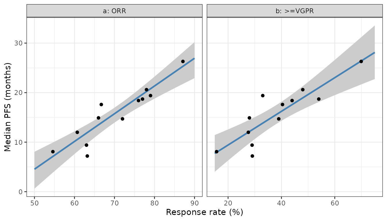
Replicates Figure 1 of Teng 2018: the blue line is the encoded model and the grey band the 95% confidence interval of the regression line.
4. Figure 2: the probability-of-technical-success example
The paper’s worked example assumes a phase II study of 50 patients
and a phase III design with a target-product-profile (TPP) median PFS of
15 months and a minimal detectable value (MDV) of 12.6 months. The ORR
model carries steps 1 and 2 of that framework: mpfs is the
predicted median PFS and mpfs_se the standard error that
comes from the binomial sampling error of the phase II ORR. Step 3 is
the normal tail probability.
pts_in <- data.frame(id = 1:2, time = 0, evid = 0, amt = NA_real_,
                     RESP_ORR_PCT = 66, N_ARM = 50)
pts_out <- suppressWarnings(rxSolve(
  rxode2::zeroRe(mod_orr, "sigma"), pts_in, returnType = "data.frame"
))[1, ]

pts_tbl <- data.frame(
  quantity = c("Predicted median PFS (months)", "P(median PFS > 15 months, TPP)",
               "P(median PFS > 12.6 months, MDV)", "ORR needed for a median PFS of 13.5 months (%)"),
  published = c(13.50, 0.34, 0.60, 66),
  model = c(
    pts_out$mpfs,
    1 - pnorm(15, pts_out$mpfs, pts_out$mpfs_se),
    1 - pnorm(12.6, pts_out$mpfs, pts_out$mpfs_se),
    (13.5 - ini_val(ui_orr, "int_mpfs")) / ini_val(ui_orr, "e_orr_mpfs")
  ),
  # The probabilities are printed as whole percentages: 0.5948 is printed as
  # 60%, so they are compared within one percentage point rather than by
  # rounding to two decimals.
  tolerance = c(0.005, 0.01, 0.01, 0.5)
)
pts_tbl$match <- abs(pts_tbl$model - pts_tbl$published) <= pts_tbl$tolerance

pts_tbl |>
  dplyr::select(-tolerance) |>
  dplyr::rename("Quantity" = quantity, "Published" = published, "Model" = model,
                "Matches the printed value" = match) |>
knitr::kable(digits = 4, caption = "Teng 2018 Figure 2 and Results, 'Relationship between response rates and PFS'.")| Quantity | Published | Model | Matches the printed value |
|---|---|---|---|
| Predicted median PFS (months) | 13.50 | 13.5000 | TRUE |
| P(median PFS > 15 months, TPP) | 0.34 | 0.3446 | TRUE |
| P(median PFS > 12.6 months, MDV) | 0.60 | 0.5948 | TRUE |
| ORR needed for a median PFS of 13.5 months (%) | 66.00 | 66.0000 | TRUE |
dens <- data.frame(pfs = seq(0, 28, by = 0.05))
dens$d <- dnorm(dens$pfs, pts_out$mpfs, pts_out$mpfs_se)
ggplot(dens, aes(pfs, d)) +
  geom_area(data = dplyr::filter(dens, pfs >= 12.6), fill = "lightblue") +
  geom_area(data = dplyr::filter(dens, pfs >= 15), fill = "orchid") +
  geom_line() +
  geom_vline(xintercept = c(12.6, 15), linetype = "dashed") +
  labs(x = "Predicted phase III median PFS (months)", y = "Density",
       title = "ORR = 66%, N = 50") +
  theme_bw()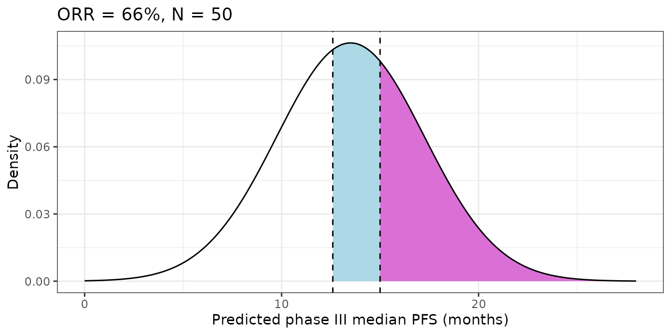
Replicates Figure 2 of Teng 2018: the purple area is the 34% probability of reaching the TPP median PFS of 15 months, and purple plus blue the 60% probability of reaching the MDV of 12.6 months.
5. Predictive check of the between-arm residual
A stochastic solve draws each arm’s median PFS around the regression
line with the derived residual SD. With 200 replicate arms at each of
the 12 fitted ORRs, the spread of the draws should recover
addSd, and the observed arms should fall inside the
simulated 90% interval at roughly the nominal rate.
n_rep <- 200
vpc_in <- arms[rep(seq_len(nrow(arms)), each = n_rep), ] |>
  dplyr::mutate(arm_row = rep(seq_len(nrow(arms)), each = n_rep),
                id = dplyr::row_number())
rxode2::rxSetSeed(20180315)
vpc <- suppressWarnings(rxSolve(mod_orr, vpc_in[, solve_cols], returnType = "data.frame"))
vpc$arm_row <- vpc_in$arm_row[match(vpc$id, vpc_in$id)]

vpc_sum <- vpc |>
  dplyr::group_by(arm_row) |>
  dplyr::summarise(lo = quantile(sim, 0.05), med = median(sim), hi = quantile(sim, 0.95),
                   .groups = "drop") |>
  dplyr::mutate(orr = arms$orr[arm_row], obs = arms$pfs[arm_row])

resid_sd <- sd(vpc$sim - vpc$ipredSim)
inside <- mean(vpc_sum$obs >= vpc_sum$lo & vpc_sum$obs <= vpc_sum$hi)

ggplot(vpc_sum, aes(orr)) +
  geom_errorbar(aes(ymin = lo, ymax = hi), width = 0.8, colour = "grey50") +
  geom_point(aes(y = med), colour = "steelblue") +
  geom_point(aes(y = obs), colour = "firebrick", shape = 17, size = 2.5) +
  labs(x = "Overall response rate (%)", y = "Median PFS (months)",
       caption = "Blue: simulated median; bars: simulated 90% interval; red: observed arm (Table 1).") +
  theme_bw()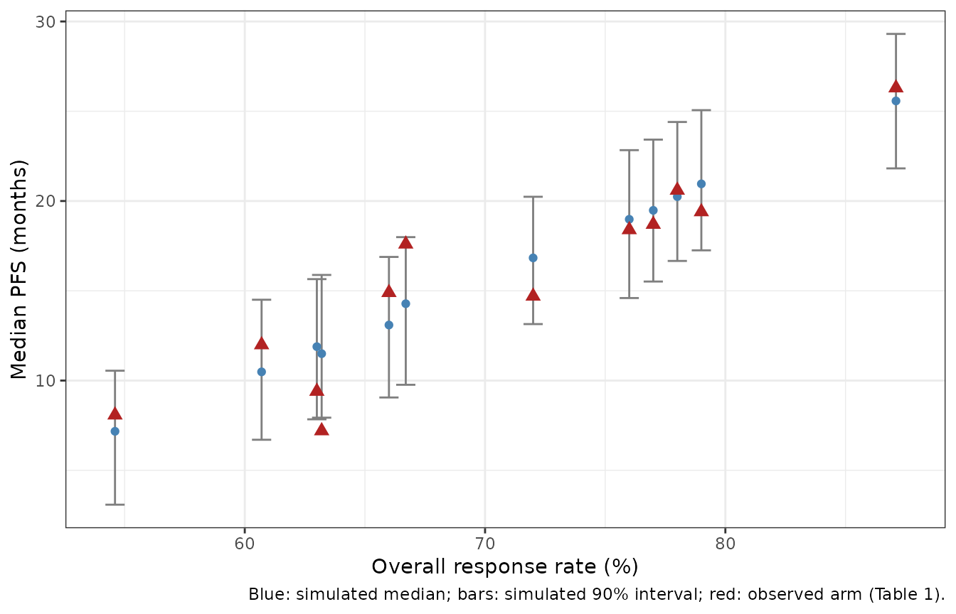
stopifnot(
  # 2,400 draws: the sample SD is within a few percent of addSd.
  abs(resid_sd / ini_val(ui_orr, "addSd") - 1) < 0.1,
  # 12 arms at a nominal 90%: allow for the small count.
  inside >= 0.75
)
The simulated residual SD is 2.36 months against an encoded 2.3472, and 11 of 12 observed arms fall inside the simulated 90% interval.
Assumptions and deviations
-
The residual SD is derived, not printed. Teng 2018
reports only R^2.
addSdis the OLS residual standard error (10 degrees of freedom) of refitting the paper’s own Table 1 with the paper’s own stated estimator, a refit that reproduces every printed coefficient (Section 1). It is annotated as derived in both model files. Nothing was substituted from outside the paper. - Printed rather than refit coefficients. The models carry the two-decimal coefficients the paper prints (-23.46, 0.56; 2.62, 0.34), not the unrounded refit (-23.4612, 0.5559; 2.6193, 0.3405). At ORR 78% the two differ by 0.3 months.
-
mpfs_secarries only the phase II sampling error. That is the paper’s step 1-2 framework exactly: it treats the regression line as known and propagates only the binomial error of the observed ORR. The regression’s own parameter and residual uncertainty are not inmpfs_se; the Bayesian layer below was the paper’s attempt to add them. - The Bayesian probability-of-technical-success layer is not encoded. Table 2 and Figure 3 place a prior N((15.61, 0.56), diag(sigma^2, sigma^2)) on the centred intercept and slope with sigma^2 ~ Inverse Gamma(10, 100). The paper does not say how this prior is combined with the residual and the phase II sampling error, and a single sigma^2 of mean about 11 on both the intercept and the per-percent slope cannot be read literally (a slope SD of about 3.3 months per percentage point would swamp the 0.56 estimate). Its Table 2 probabilities (for example 28% at ORR 66%, against 34% from the frequentist Figure 2) are therefore not reproduced. Figure 4’s alternative approach evaluates “equation (8) in Hong and Shi (2012)” (Stat Med 31:831-843), which was not available when the model was built. Neither layer is a model parameter; both are decision-analysis wrappers around the same regression.
- Figure 2 caption. The caption says “for an ORR of 60%”, but the figure panel, the Results text and the arithmetic all give 66% (-23.46 + 0.56 * 66 = 13.50 months). The vignette uses 66%.
- No between-study random effect. The source is unweighted OLS, so the models carry no eta and do not weight arms by size; two arms of one trial are treated as independent.
-
Range of use. The paper recommends prediction only
for an observed ORR of 50-85% (fitted range 54.6-87.1%), and the normal
approximation in
mpfs_seneeds at least five responders and five non-responders. - Response criteria are pooled. PANORAMA-1 and ELOQUENT-2 assessed response by EBMT criteria and the other five trials by IMWG criteria; the paper pools them, and so do the models.