Anti-VEGF therapy in neovascular AMD (Luu 2022)
Source:vignettes/articles/Luu_2022_antiVegf.Rmd
Luu_2022_antiVegf.RmdModel and source
- Citation: Luu KT, Seal J, Green M, Winskill C, Attar M. Effect of Anti-VEGF Therapy on the Disease Progression of Neovascular Age-Related Macular Degeneration: A Systematic Review and Model-Based Meta-Analysis. J Clin Pharmacol. 2022;62(5):594-608. doi:10.1002/jcph.2002. PMCID: PMC9305109.
- Description: MBMA. Model-based meta-analysis of best-corrected visual acuity (SCORE_BCVA, ETDRS letters) in neovascular age-related macular degeneration (nAMD) under intravitreal anti-VEGF therapy with ranibizumab, aflibercept, brolucizumab or abicipar, or under sham, fitted to study-arm-level aggregate data from 22 randomised trials (55 arms, 9548 subjects) (Luu 2022). Natural disease progression is an indirect-response model in which SCORE_BCVA declines from its baseline toward a steady state gss = kin/kout; each drug stimulates kin through C/(EC50 + C) with a maximal effect Emax_ss * (1 + dEmax0 * exp(-kEmax * t)) that is largest at treatment onset. Vitreous PK is one compartment (4 mL) with first-order elimination at a fixed, drug-specific half-life; vitreous concentration is converted to nM with the molecular weight of each drug, and EC50 is drug-specific. The drug in an arm is selected by the TRT_RANIBIZUMAB / TRT_AFLIBERCEPT / TRT_BROLUCIZUMAB / TRT_ABICIPAR indicators (all 0 = sham). Arm-average baseline SCORE_BCVA (centred at 56.4 letters) is a covariate on the kout half-life (power) and on Emax_ss (on the logit scale). Between-arm variability is on the kout half-life, logit Emax_ss and dEmax0. The residual is additive in letters with separate SDs for sham arms, for treated arms in the first year and for treated arms after the first year, each divided by sqrt(N_ARM). Suitable scope is arm-mean SCORE_BCVA trajectories, NOT individual patients. Bevacizumab arms were in the fitted data but have no published half-life and are not supported.
- Article (open access): https://doi.org/10.1002/jcph.2002
Luu 2022 is a model-based meta-analysis (MBMA) of arm-mean
best-corrected visual acuity (BCVA, ETDRS letters) in neovascular
age-related macular degeneration. It extends the individual-level
ranibizumab model of Mulyukov 2018 (packaged as
Mulyukov_2018_ranibizumab) to four anti-VEGF agents and to
sham arms. It then uses the model for a virtual head-to-head comparison
of every-12-week (Q12) dosing.
Population
The analysis data set holds 22 randomised trials with 55 monotherapy or sham arms and 9548 subjects (Luu 2022 Table 2): ANCHOR, BAMBOO, BRAMD, C-10-083, C-12-006, CANTREAT, CATT, CEDAR, CYPRESS, EOP1003, EOP1004, EXCITE, HAGA, HARRIER, HAWK, MARINA, MORI, PIER, REACH, SEQUOIA, VIEW 1 and VIEW 2. Trial length was 4.33 to 104 weeks. Arm-average baseline BCVA was 47.0 to 65.8 letters, with a median of 56.4 letters over the 55 arms. Only aggregate arm data were used. The paper reports no age, sex or race distribution. Arms with pro re nata or treat-and-extend dosing were excluded. The two bevacizumab arms were fitted but could not be simulated, because no bevacizumab half-life or EC50 was estimated.
The same information is available programmatically via
readModelDb("Luu_2022_antiVegf_mbma")()$population.
Source trace
| Equation / parameter | Value | Source location |
|---|---|---|
d/dt(bcva) |
kin * (1 + Emax_ss * (1 + dEmax0 * exp(-kEmax * t)) * C / (EC50 + C)) - kout * bcva |
Luu 2022 Eq 1, p. 596 |
kin |
gss * kout |
Luu 2022 Methods, text below Eq 1 (gss = kin/kout) |
d/dt(central) |
-kel * central |
Luu 2022 Eq 2, p. 596 |
lvvit |
log(0.004 L) | Methods: vitreous volume 4 mL |
lgss |
log(35.4 letters) | Table 1 g ss
|
lthalf_kout |
log(21.6 week) | Table 1 HL_kout
|
lthalf_ranibizumab |
log(1.29 week), fixed | Table 1 HL_Rani
|
lthalf_brolucizumab |
log(0.629 week), fixed | Table 1 HL_Bro
|
lthalf_aflibercept |
log(0.786 week), fixed | Table 1 HL_Aflib
|
lthalf_abicipar |
log(0.649 week), fixed | Table 1 HL_Abic
|
logitemaxss |
logit(0.842) | Table 1 Emax ss
|
ldemax0 |
log(5.87) | Table 1 Delta Emax 0
|
lthalf_kemax |
log(0.494 week) | Table 1 HL_kEmax
|
lec50_ranibizumab |
log(14.7 nM) | Table 1 Ra_EC50
|
lec50_aflibercept |
log(1.12 nM) | Table 1 Af_EC50
|
lec50_abicipar |
log(0.0308 nM) | Table 1 Ab_EC50
|
lec50_brolucizumab |
log(0.0026 nM) | Table 1 Br_EC50
|
e_score_bcva_thalf_kout |
2.57 | Table 1 Base_HL_kout
|
e_score_bcva_emaxss |
2.00 | Table 1 Base_Emax
|
eta_arm_thalf_kout |
0.99^2 | Table 1 between-arm variability HL_kout 99% |
eta_arm_emaxss |
0.0935^2 | Table 1 between-arm variability Emax 9.35% |
eta_arm_demax0 |
1.18^2 | Table 1 between-arm variability Delta Emax 118% |
addSd |
5.2 letters | Table 1 Sigma 1 (treatment) |
addSd_late |
4.84 letters | Table 1 Sigma 2 (treatment, after year 1) |
addSd_sham |
6.64 letters | Table 1 Sigma 3 (sham) |
residual / sqrt(N_ARM) |
n/a | Methods: residual weighted by the square root of the number of subjects |
| molecular weights 48 / 115 / 26 / 34 kDa | n/a | Lucentis, Eylea (Luu 2022 ref 32) and Beovu labels; Callanan 2018 (Luu 2022 ref 16) |
| centring 56.4 letters | n/a | median of the 55 arm baselines of Table 2 |
Virtual arms
The model describes trial-arm means, so each simulated “subject” below is one trial arm. The arm list reproduces the regimens and baseline BCVA of Luu 2022 Table 2 for the regimen groups shown in Figure 4. “Monthly” dosing (Table 2 footnote a) is every 52/12 weeks, and Q4 is every 4 weeks.
monthly <- 52 / 12
regimens <- list(
  rani_monthly = seq(0, 52, by = monthly),
  q4 = seq(0, 48, by = 4),
  # Three monthly loading doses, then every 3 months (EXCITE, PIER).
  rani_q12 = c(0, 1, 2, 5, 8, 11) * monthly,
  # Three 4-weekly loading doses, then every 12 weeks (HAWK, HARRIER).
  bro_q12 = c(0, 4, 8, 20, 32, 44),
  # Three 4-weekly loading doses, then every 8 weeks.
  q8 = c(0, 4, 8, 16, 24, 32, 40, 48),
  # Loading doses at weeks 0, 4 and 12, then every 12 weeks (Figure 5).
  q12 = c(0, 4, 12, 24, 36, 48)
)

# One row per Figure 4 regimen group: drug, dose (mg), regimen, the baseline
# BCVA of each contributing Table 2 arm, the assessment week, and the
# Figure 4 model-predicted and observed week 48/52 change from baseline.
fig4 <- tibble::tribble(
  ~group, ~drug, ~dose, ~regimen, ~base, ~week, ~pred_paper, ~obs_paper,
  "Ranibizumab, monthly (0.5 mg)", "ranibizumab", 0.5, "rani_monthly", c(47.1, 60.0, 59.5, 53.7, 53.8), 52, 7.42, 7.43,
  "Ranibizumab, monthly (0.3 mg)", "ranibizumab", 0.3, "rani_monthly", c(47.0, 53.1, 56.5), 52, 7.31, 7.42,
  "Ranibizumab, Q4 (0.5 mg)", "ranibizumab", 0.5, "q4", c(60.1, 56.4, 57.0, 54.0), 52, 8.70, 8.59,
  "Ranibizumab, Q12 (0.5 mg)", "ranibizumab", 0.5, "rani_q12", c(57.7, 53.7), 52, 2.77, 1.78,
  "Ranibizumab, Q12 (0.3 mg)", "ranibizumab", 0.3, "rani_q12", c(55.8, 55.8), 52, 2.31, 2.13,
  "Brolucizumab, Q12/Q8 (6 mg)", "brolucizumab", 6, "bro_q12", c(60.8, 61.5), 48, 6.74, 6.75,
  "Brolucizumab, Q12/Q8 (3 mg)", "brolucizumab", 3, "bro_q12", c(61.0), 48, 6.23, 6.10,
  "Aflibercept, Q8 (2 mg)", "aflibercept", 2, "q8", c(55.7, 51.6, 60.0, 60.8, 63.1, 65.8), 52, 7.75, 7.83,
  "Aflibercept, Q4 (2 mg)", "aflibercept", 2, "q4", c(55.2, 52.8), 52, 9.06, 9.24,
  "Aflibercept, Q4 (0.5 mg)", "aflibercept", 0.5, "q4", c(55.6, 51.6), 52, 8.44, 8.24,
  "Abicipar, Q8 (2 mg)", "abicipar", 2, "q8", c(56.5, 57.2), 52, 7.47, 7.49,
  "Abicipar, Q12 (2 mg)", "abicipar", 2, "q12", c(56.4, 56.4), 52, 5.92, 6.12
)

# Build the event table for one arm. Doses go into the vitreous `central`
# compartment; observations are on the `bcva` state.
make_arm <- function(id, drug, dose, dose_times, base, week, n_arm = 300,
                     obs_times = c(0, week)) {
  trt <- c(ranibizumab = 0, aflibercept = 0, brolucizumab = 0, abicipar = 0)
  if (drug != "sham") trt[[drug]] <- 1
  doses <- if (drug == "sham") NULL else
    tibble(time = dose_times[dose_times < week], evid = 1L, amt = dose, cmt = "central")
  bind_rows(doses, tibble(time = obs_times, evid = 0L, amt = 0, cmt = "bcva")) |>
    mutate(
      id = id,
      TRT_RANIBIZUMAB = trt[["ranibizumab"]],
      TRT_AFLIBERCEPT = trt[["aflibercept"]],
      TRT_BROLUCIZUMAB = trt[["brolucizumab"]],
      TRT_ABICIPAR = trt[["abicipar"]],
      SCORE_BCVA = base,
      N_ARM = n_arm
    ) |>
    arrange(time, desc(evid))
}

arms4 <- fig4 |>
  mutate(g = row_number()) |>
  tidyr::unnest(base) |>
  mutate(id = row_number())
ev4 <- bind_rows(lapply(seq_len(nrow(arms4)), function(i) {
  a <- arms4[i, ]
  make_arm(a$id, a$drug, a$dose, regimens[[a$regimen]], a$base, a$week) |>
    mutate(group = a$group)
}))
stopifnot(!anyDuplicated(unique(ev4[, c("id", "time", "evid")])))
Simulation
mod <- readModelDb("Luu_2022_antiVegf_mbma")
mod_typical <- rxode2::zeroRe(mod, "omega")
#> ℹ parameter labels from comments will be replaced by 'label()'

# Each simulated id is one trial arm, so a typical-value solve over several
# arms is intended; muffle only rxode2's warning about that.
solve_typical <- function(events, ...) {
  withCallingHandlers(
    rxode2::rxSolve(mod_typical, events = events, ...),
    warning = function(w) {
      if (grepl("without 'omega'", conditionMessage(w), fixed = TRUE)) {
        invokeRestart("muffleWarning")
      }
    }
  )
}
sim4 <- solve_typical(ev4, keep = "group") |>
  as.data.frame()
#> ℹ omega/sigma items treated as zero: 'eta_arm_thalf_kout', 'eta_arm_emaxss', 'eta_arm_demax0'
Replicate published figures
Figure 4: week 48/52 change from baseline on the labelled regimens
Luu 2022 Figure 4 compares, for each regimen group, the observed mean change from baseline with the mean model prediction across the contributing arms. The paper’s predictions use each arm’s empirical Bayes estimates (Results, p. 600). The library model has no arm estimates, so the values below are typical-value predictions at each arm’s baseline BCVA, averaged over the arms of the group.
fig4_sim <- sim4 |>
  group_by(id, group) |>
  filter(time == max(time)) |>
  ungroup() |>
  group_by(group) |>
  summarise(cfb_sim = mean(bcva_cfb), .groups = "drop") |>
  left_join(select(fig4, group, pred_paper, obs_paper), by = "group") |>
  mutate(diff = cfb_sim - pred_paper)
stopifnot(nrow(fig4_sim) == nrow(fig4))

fig4_sim |>
  mutate(across(c(cfb_sim, diff), \(x) round(x, 2))) |>
  rename(
    "Regimen group" = group,
    "Simulated typical value (letters)" = cfb_sim,
    "Luu 2022 predicted (letters)" = pred_paper,
    "Luu 2022 observed (letters)" = obs_paper,
    "Simulated - predicted" = diff
  ) |>
knitr::kable(caption = "Replicates Figure 4 of Luu 2022: mean change from baseline BCVA at week 48 (brolucizumab) or 52.")| Regimen group | Simulated typical value (letters) | Luu 2022 predicted (letters) | Luu 2022 observed (letters) | Simulated - predicted |
|---|---|---|---|---|
| Abicipar, Q12 (2 mg) | 6.98 | 5.92 | 6.12 | 1.06 |
| Abicipar, Q8 (2 mg) | 7.55 | 7.47 | 7.49 | 0.08 |
| Aflibercept, Q4 (0.5 mg) | 9.92 | 8.44 | 8.24 | 1.48 |
| Aflibercept, Q4 (2 mg) | 9.76 | 9.06 | 9.24 | 0.70 |
| Aflibercept, Q8 (2 mg) | 5.04 | 7.75 | 7.83 | -2.71 |
| Brolucizumab, Q12/Q8 (3 mg) | 4.41 | 6.23 | 6.10 | -1.82 |
| Brolucizumab, Q12/Q8 (6 mg) | 4.35 | 6.74 | 6.75 | -2.39 |
| Ranibizumab, Q12 (0.3 mg) | 1.11 | 2.31 | 2.13 | -1.20 |
| Ranibizumab, Q12 (0.5 mg) | 2.57 | 2.77 | 1.78 | -0.20 |
| Ranibizumab, Q4 (0.5 mg) | 7.16 | 8.70 | 8.59 | -1.54 |
| Ranibizumab, monthly (0.3 mg) | 10.47 | 7.31 | 7.42 | 3.16 |
| Ranibizumab, monthly (0.5 mg) | 8.77 | 7.42 | 7.43 | 1.35 |
# Deterministic typical values. Realised: median |diff| 1.42 letters, mean
# signed diff -0.01, max |diff| 3.16 (ranibizumab monthly 0.3 mg, whose ANCHOR
# arm starts at 47 letters). A tenfold EC50 error or a swapped half-life moves
# several groups by more than 3 letters and the mean by more than 1.
stopifnot(
  median(abs(fig4_sim$diff)) < 2,
  abs(mean(fig4_sim$diff)) < 1
)
fig4_sim |>
  select(group, `Simulated typical value` = cfb_sim, `Luu 2022 predicted` = pred_paper,
         `Luu 2022 observed` = obs_paper) |>
  pivot_longer(-group, names_to = "source", values_to = "cfb") |>
  ggplot(aes(cfb, group, colour = source)) +
  geom_point(size = 2.5) +
  labs(x = "Change from baseline at week 48/52 (letters)", y = NULL, colour = NULL,
       caption = "Replicates Figure 4 of Luu 2022.") +
  theme(legend.position = "bottom")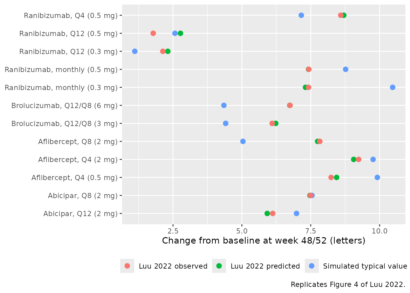
Figure 5: virtual head-to-head comparison of Q12 dosing
Figure 5 simulates each drug with loading doses at weeks 0, 4 and 12 and then every 12 weeks, at the baseline BCVA of every arm of that drug in Table 2. Doses are the labelled strengths: abicipar 2 mg, aflibercept 2 mg, brolucizumab 6 mg and ranibizumab 0.5 mg.
base5 <- list(
  abicipar = c(58.5, 54.3, 56.4, 56.5, 55.2, 59.0, 58.4, 58.5, 56.4, 57.2),
  aflibercept = c(55.6, 63.1, 60.8, 60.0, 65.8, 55.2, 55.6, 55.7, 52.8, 51.6, 51.6),
  brolucizumab = c(63.6, 57.9, 56.8, 54.9, 54.1, 61.5, 61.0, 60.8),
  ranibizumab = c(47.0, 47.1, 55.8, 60.0, 56.6, 59.5, 60.1, 56.4, 57.6, 55.8,
                  57.7, 56.5, 53.1, 53.7, 55.8, 53.7, 60.4, 57.0, 54.0, 53.8)
)
dose5 <- c(abicipar = 2, aflibercept = 2, brolucizumab = 6, ranibizumab = 0.5)
arms5 <- tibble(drug = names(base5), base = base5) |>
  tidyr::unnest(base) |>
  mutate(id = row_number())
ev5 <- bind_rows(lapply(seq_len(nrow(arms5)), function(i) {
  a <- arms5[i, ]
  make_arm(a$id, a$drug, dose5[[a$drug]], regimens$q12, a$base, 52,
           obs_times = 0:52) |>
    mutate(drug = a$drug)
}))
sim5 <- solve_typical(ev5, keep = "drug") |>
  as.data.frame()
#> ℹ omega/sigma items treated as zero: 'eta_arm_thalf_kout', 'eta_arm_emaxss', 'eta_arm_demax0'

fig5_paper <- tibble::tribble(
  ~drug, ~mean_paper, ~sd_paper,
  "abicipar", 5.92, 1.02,
  "aflibercept", 3.04, 1.61,
  "brolucizumab", 6.61, 0.284,
  "ranibizumab", 3.02, 2.35
)
fig5_sim <- sim5 |>
  filter(time == 52) |>
  group_by(drug) |>
  summarise(mean_sim = mean(bcva_cfb), sd_sim = sd(bcva_cfb), .groups = "drop") |>
  left_join(fig5_paper, by = "drug") |>
  mutate(diff = mean_sim - mean_paper)
stopifnot(nrow(fig5_sim) == 4)

fig5_sim |>
  mutate(across(c(mean_sim, sd_sim, diff), \(x) round(x, 2))) |>
  rename(
    "Drug" = drug,
    "Simulated mean (letters)" = mean_sim,
    "Simulated SD across arms" = sd_sim,
    "Luu 2022 mean (letters)" = mean_paper,
    "Luu 2022 SD" = sd_paper,
    "Simulated - Luu 2022" = diff
  ) |>
knitr::kable(caption = "Replicates Figure 5 of Luu 2022: week 52 change from baseline on fixed Q12 dosing.")| Drug | Simulated mean (letters) | Simulated SD across arms | Luu 2022 mean (letters) | Luu 2022 SD | Simulated - Luu 2022 |
|---|---|---|---|---|---|
| abicipar | 6.52 | 1.17 | 5.92 | 1.020 | 0.60 |
| aflibercept | 2.91 | 3.10 | 3.04 | 1.610 | -0.13 |
| brolucizumab | 6.13 | 2.51 | 6.61 | 0.284 | -0.48 |
| ranibizumab | 3.68 | 2.66 | 3.02 | 2.350 | 0.66 |
# Deterministic. Realised |diff| 0.13-0.66 letters. The paper's conclusion
# that abicipar and brolucizumab keep about 3 more letters than aflibercept
# and ranibizumab on Q12 dosing is checked as a gap, not as an ordering of
# near-equal values.
cfb5 <- setNames(fig5_sim$mean_sim, fig5_sim$drug)
stopifnot(
  all(abs(fig5_sim$diff) < 1.2),
  min(cfb5[c("abicipar", "brolucizumab")]) - max(cfb5[c("aflibercept", "ranibizumab")]) > 1.5
)
sim5 |>
  group_by(drug, time) |>
  summarise(cfb = mean(bcva_cfb), .groups = "drop") |>
  ggplot(aes(time, cfb, colour = drug)) +
  geom_line(linewidth = 0.8) +
  geom_vline(xintercept = regimens$q12, linetype = "dotted", colour = "grey50") +
  labs(x = "Time from first dose (weeks)", y = "Change from baseline BCVA (letters)",
       colour = NULL,
       caption = "Mean typical-value trajectory across the Table 2 arms of each drug; Q12 dosing as in Figure 5 of Luu 2022.")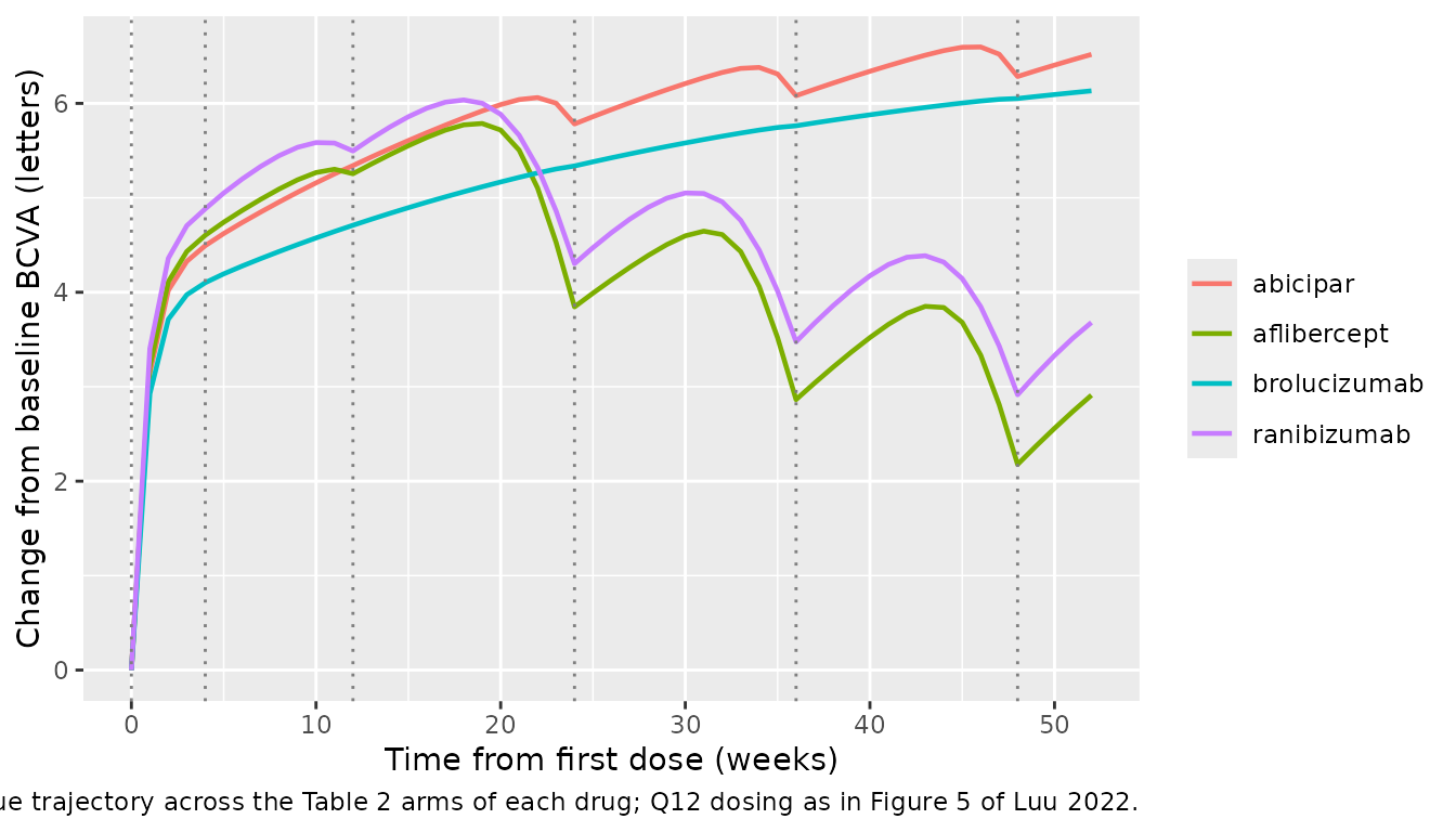
Natural disease progression (sham)
Without treatment, BCVA declines from its baseline toward
gss = 35.4 letters with half-life HL_kout (Luu
2022 Eq 1 with C = 0). The ODE solution is checked against the closed
form g(t) = gss + (g0 - gss) * exp(-kout * t).
sham_base <- c(EOP1003 = 51.3, EOP1004 = 54.0, MARINA = 53.6, PIER = 55.1)
ev_sham <- bind_rows(lapply(seq_along(sham_base), function(i) {
  make_arm(i, "sham", 0, NULL, sham_base[[i]], 104, obs_times = seq(0, 104, by = 2)) |>
    mutate(trial = names(sham_base)[i])
}))
sim_sham <- solve_typical(ev_sham, keep = "trial") |>
  as.data.frame()
#> ℹ omega/sigma items treated as zero: 'eta_arm_thalf_kout', 'eta_arm_emaxss', 'eta_arm_demax0'

closed <- sim_sham |>
  mutate(
    g0 = sham_base[trial],
    kout = log(2) / (21.6 * (g0 / 56.4)^2.57),
    g_closed = 35.4 + (g0 - 35.4) * exp(-kout * time)
  )
# Same parameters on both sides, so the difference is integrator error only.
stopifnot(max(abs(closed$bcva - closed$g_closed)) < 1e-3)

ggplot(sim_sham, aes(time, bcva_cfb, colour = trial)) +
  geom_line() +
  labs(x = "Time (weeks)", y = "Change from baseline BCVA (letters)", colour = "Sham arm",
       caption = "Typical-value sham trajectories at the Table 2 baselines (compare Figure 2F of Luu 2022).")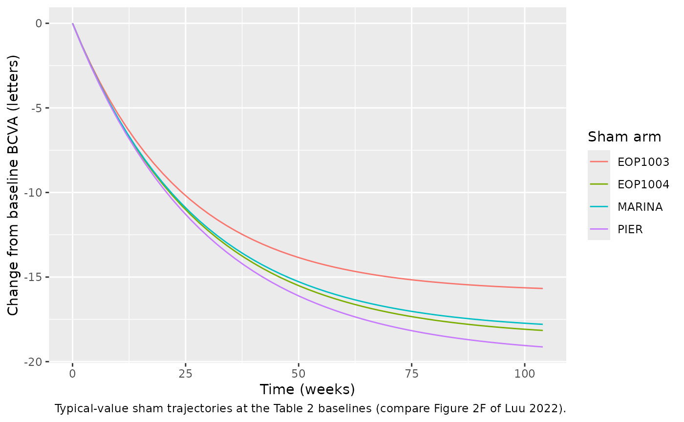
Between-arm variability
A stochastic simulation of 200 virtual ranibizumab 0.5 mg Q4 arms at
the median baseline (56.4 letters) shows the spread implied by the
between-arm variability on HL_kout, Emax_ss
and dEmax0. The plotted quantity is the arm-level
prediction without residual error; for an arm of 300 subjects the
residual adds an SD of only 5.2 / sqrt(300) = 0.3 letters.
ev_vpc <- bind_rows(lapply(1:200, function(i) {
  make_arm(i, "ranibizumab", 0.5, regimens$q4, 56.4, 52, obs_times = seq(0, 52, by = 2))
}))
rxode2::rxSetSeed(2022)
sim_vpc <- rxode2::rxSolve(mod, events = ev_vpc) |> as.data.frame()
#> ℹ parameter labels from comments will be replaced by 'label()'

vpc <- sim_vpc |>
  group_by(time) |>
  summarise(
    Q05 = quantile(bcva_cfb, 0.05),
    Q50 = quantile(bcva_cfb, 0.50),
    Q95 = quantile(bcva_cfb, 0.95),
    .groups = "drop"
  )
typ <- solve_typical(filter(ev_vpc, id == 1)) |> as.data.frame()
#> ℹ omega/sigma items treated as zero: 'eta_arm_thalf_kout', 'eta_arm_emaxss', 'eta_arm_demax0'

# Centre only. A misplaced eta or a variance read as a CV shifts the median
# arm by several letters.
stopifnot(abs(vpc$Q50[vpc$time == 52] - typ$bcva_cfb[typ$time == 52]) < 2.5)

ggplot(vpc, aes(time, Q50)) +
  geom_ribbon(aes(ymin = Q05, ymax = Q95), alpha = 0.25) +
  geom_line() +
  geom_line(data = typ, aes(time, bcva_cfb), linetype = "dashed", colour = "blue") +
  labs(x = "Time (weeks)", y = "Change from baseline BCVA (letters)",
       caption = "Median and 90% interval of 200 simulated ranibizumab 0.5 mg Q4 arms; dashed: typical value.")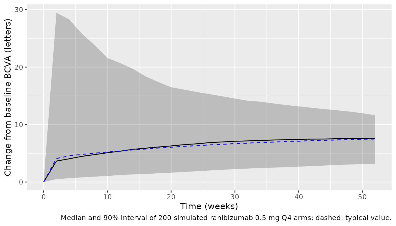
PKNCA validation of the vitreous PK
The vitreous PK is one compartment with a fixed, drug-specific half-life. A single labelled dose of each drug is checked with PKNCA. Cmax should equal dose / 4 mL and the terminal half-life should equal the Table 1 value.
pk_dose <- c(ranibizumab = 0.5, aflibercept = 2, brolucizumab = 6, abicipar = 2)
ev_pk <- bind_rows(lapply(seq_along(pk_dose), function(i) {
  d <- names(pk_dose)[i]
  make_arm(i, d, pk_dose[[d]], 0, 56.4, 12, obs_times = c(0, 0.05, 0.1, 0.25, 0.5, 1:12)) |>
    mutate(treatment = d)
}))
sim_pk <- solve_typical(ev_pk, keep = "treatment") |>
  as.data.frame()
#> ℹ omega/sigma items treated as zero: 'eta_arm_thalf_kout', 'eta_arm_emaxss', 'eta_arm_demax0'

sim_nca <- sim_pk |>
  filter(!is.na(Cc)) |>
  select(id, time, Cc, treatment)
dose_df <- ev_pk |>
  filter(evid == 1) |>
  select(id, time, amt, treatment)

conc_obj <- PKNCA::PKNCAconc(sim_nca, Cc ~ time | treatment + id)
dose_obj <- PKNCA::PKNCAdose(dose_df, amt ~ time | treatment + id, route = "intravascular")
intervals <- data.frame(start = 0, end = Inf, cmax = TRUE, tmax = TRUE,
                        aucinf.obs = TRUE, half.life = TRUE)
nca_res <- PKNCA::pk.nca(PKNCA::PKNCAdata(conc_obj, dose_obj, intervals = intervals))

published <- tibble::tribble(
  ~treatment, ~cmax, ~half.life,
  "ranibizumab", 0.5 / 0.004, 1.29,
  "aflibercept", 2 / 0.004, 0.786,
  "brolucizumab", 6 / 0.004, 0.629,
  "abicipar", 2 / 0.004, 0.649
)
cmp <- nlmixr2lib::ncaComparisonTable(
  simulated = nca_res,
  reference = published,
  by = "treatment",
  units = c(cmax = "mg/L", half.life = "week"),
  tolerance_pct = 20
)
knitr::kable(cmp, caption = "Simulated vitreous NCA vs. dose / 4 mL and the Table 1 half-lives. * differs by >20%.")| NCA parameter | treatment | Reference | Simulated | % diff |
|---|---|---|---|---|
| Cmax (mg/L) | ranibizumab | 125 | 125 | +0.0% |
| Cmax (mg/L) | aflibercept | 500 | 500 | +0.0% |
| Cmax (mg/L) | brolucizumab | 1500 | 1500 | +0.0% |
| Cmax (mg/L) | abicipar | 500 | 500 | +0.0% |
| t½ (week) | ranibizumab | 1.29 | 1.29 | -0.0% |
| t½ (week) | aflibercept | 0.786 | 0.786 | -0.0% |
| t½ (week) | brolucizumab | 0.629 | 0.629 | +0.0% |
| t½ (week) | abicipar | 0.649 | 0.649 | -0.0% |
nca_tab <- as.data.frame(nca_res$result) |>
  filter(PPTESTCD %in% c("cmax", "half.life")) |>
  select(treatment, PPTESTCD, PPORRES) |>
  pivot_wider(names_from = PPTESTCD, values_from = PPORRES) |>
  left_join(published, by = "treatment", suffix = c("_sim", "_ref"))
# Closed-form one-compartment PK, so only integration error separates the sides.
stopifnot(
  nrow(nca_tab) == 4,
  all(abs(nca_tab$cmax_sim / nca_tab$cmax_ref - 1) < 1e-3),
  all(abs(nca_tab$half.life_sim / nca_tab$half.life_ref - 1) < 1e-3)
)
The drug effect is driven by the vitreous concentration in nM,
Cc * 1000 / MW(kDa). For example, 0.5 mg ranibizumab gives
125 mg/L / 48 kDa = 2604 nM, about 180 times its EC50 of 14.7 nM.
Assumptions and deviations
- Molecular weights are not printed in Luu 2022. EC50 values are in nM, so each vitreous concentration is converted from mg/L with the molecular weight of its drug. The maintainers took the weights from the sources the paper cites: ranibizumab ~48 kDa (Lucentis label), aflibercept 115 kDa including glycosylation (Eylea label, Luu 2022 ref 32), brolucizumab ~26 kDa (Beovu label) and abicipar 34 kDa (Callanan 2018, Luu 2022 ref 16). With these, the typical-value model reproduces the Figure 5 Q12 predictions to within 0.7 letters.
- Covariate centring. The paper centres continuous covariates “on a typical value, eg, the median of the study population” but does not print the value. The model uses 56.4 letters, the median of the 55 arm baselines in Table 2.
-
Transform of the between-arm variability and form of the
baseline covariate. The paper models between-arm variability
“as additive to logit-transformed parameters” and tests covariates “in
log-space with a linear model”. A logit needs no assumed bounds only for
Emax_ss(0.842), so the maintainers ruled thatEmax_ssis logit-normal, with the baseline covariate entering on the logit scale as2.00 * log(SCORE_BCVA / 56.4). This keepsEmax_ssbelow 1 for every arm.HL_koutanddEmax0are log-normal, with a power covariate onHL_kout. The alternative reading, a multiplicative power(SCORE_BCVA / 56.4)^2.00onEmax_ss, gives typical-value Figure 4 predictions closer to the paper. It also gives Figure 5 Q12 predictions about 1.3 letters higher for brolucizumab and abicipar. Neither comparison decides between the readings, because the paper’s figures average arm-specific empirical Bayes predictions rather than typical values. Arms whose baseline is far from 56.4 letters are the most sensitive to this choice. - Between-arm variability percentages (99%, 9.35%, 118%) are read as 100 times the standard deviation of the arm random effect on the transformed scale. A coefficient of variation is undefined on the logit scale, so the same reading is applied to all three.
-
Residual error. The three additive SDs of Table 1
are used for sham arms, for treated arms up to week 52 and for treated
arms after week 52. Each is divided by
sqrt(N_ARM), following “weighted by the square root of the number of subjects”.N_ARMaffects only the residual. -
Time origin.
tinexp(-kEmax * t)is the time from the first dose (the x-axis of Figure 2), so event tables must start dosing at time 0. - Typical values, not empirical Bayes estimates. The paper’s Figures 4 and 5 average predictions that use each arm’s estimated random effects. Those estimates are not published, so this vignette compares typical-value predictions. Their across-arm SD reflects only the baseline-BCVA covariate.
- Dosing schedules. The arm regimens follow the Table 2 footnotes. For EXCITE and PIER Q12 the vignette uses three monthly loading doses, then quarterly dosing. For HAWK and HARRIER it uses three 4-weekly loading doses, then fixed Q12 dosing; the as-needed switches to Q8 are not reproduced. For Q8 regimens it uses three 4-weekly loading doses, then every 8 weeks. For abicipar Q12 it uses the Figure 5 schedule (weeks 0, 4, 12, then every 12 weeks), which gives the same 5.92-letter prediction in Figures 4 and 5.
- Bevacizumab arms (BRAMD, CATT) were fitted with the ranibizumab EC50, but no bevacizumab half-life is reported, so bevacizumab is not supported. The paper excluded it from its own simulations.
- No erratum or correction notice for Luu 2022 was found as of 2026-10-16.