Two-target (soluble + membrane) TMDD and its QSS approximation (Gibiansky 2010)
Source:vignettes/articles/Gibiansky_2010_mab_two_target_tmdd.Rmd
Gibiansky_2010_mab_two_target_tmdd.RmdModel and source
- Citation: Gibiansky L, Gibiansky E. Target-mediated drug disposition model for drugs that bind to more than one target. J Pharmacokinet Pharmacodyn. 2010;37(4):323-346.
- Article: https://doi.org/10.1007/s10928-010-9163-3
Several therapeutic antibodies bind both the soluble and the membrane-bound form of the same receptor. Gibiansky and Gibiansky extend the Mager-Jusko target-mediated drug disposition (TMDD) equations to a drug that binds any of N targets (one at a time), derive the quasi-steady-state (QSS) approximation of the multi-target system, and then specialise it to two targets: a soluble target S, kept as a QSS total-target state, and a membrane-bound target M whose total concentration is constant and small, so that it reduces to a Michaelis-Menten elimination term. A simulation-estimation study shows that this two-target QSS model (their model M3) recovers every parameter of the full model, including the unobserved membrane target, when both targets contribute comparably to elimination.
The paper contributes two models:
mod_full <- readModelDb("Gibiansky_2010_mab_two_target_tmdd_full")
mod_qss <- readModelDb("Gibiansky_2010_mab_two_target_tmdd_qss")
ui_full <- rxode2::rxode(mod_full)
#> ℹ parameter labels from comments will be replaced by 'label()'
ui_qss <- rxode2::rxode(mod_qss)
#> ℹ parameter labels from comments will be replaced by 'label()'

tibble::tibble(
  Model = c("Gibiansky_2010_mab_two_target_tmdd_full", "Gibiansky_2010_mab_two_target_tmdd_qss"),
  `Paper equations` = c("Eqs 1-3, N = 2 (the simulation 'true' model, M4)", "Eqs 12-17 (model M3)"),
  `ODE states` = c(paste(ui_full$state, collapse = ", "), paste(ui_qss$state, collapse = ", "))
) |>
knitr::kable()| Model | Paper equations | ODE states |
|---|---|---|
| Gibiansky_2010_mab_two_target_tmdd_full | Eqs 1-3, N = 2 (the simulation ‘true’ model, M4) | depot, central, peripheral1, target_soluble, target_membrane, complex_soluble, complex_membrane |
| Gibiansky_2010_mab_two_target_tmdd_qss | Eqs 12-17 (model M3) | depot, central, peripheral1, total_target_soluble |
No drug is named anywhere in the paper. The parameter values were “chosen to imitate a monoclonal antibody that binds to the soluble (S) and membrane-bound (M) targets” (Abstract).
Population
There is no observed population. The authors simulated 224 subjects from the full model in two hypothetical studies (Table 2): Study 1 with six subjects in each of four single-dose arms (100, 300 and 600 nmol i.v., 1000 nmol s.c.), and Study 2 with 100 subjects in each of two arms receiving 600 nmol i.v. or 1000 nmol s.c. on days 0, 28 and 56. The assumed inter-individual variability was 20% CV on every parameter except F, kon and koff, and the residual error was log-normal with 15% (drug) and 20% (target) CV. Concentrations below 0.1 nmol/L were removed, leaving 3,298 free-drug and 3,257 total S-target observations.
pop <- ui_full$population
tibble::tibble(
  Field = names(pop),
  Value = vapply(pop, \(x) paste(as.character(x), collapse = " "), "")
) |>
knitr::kable()| Field | Value |
|---|---|
| species | None (methodology paper; hypothetical monoclonal antibody, simulated subjects, no fitted patient data) |
| n_subjects | 224 |
| n_studies | 2 |
| disease_state | None. The parameters ‘were chosen to imitate a monoclonal antibody that binds to the soluble (S) and membrane-bound (M) targets’ (Abstract); no drug or indication is named. |
| dose_range | Study 1: single 100, 300 or 600 nmol i.v. or 1000 nmol s.c. (6 subjects per arm); Study 2: 600 nmol i.v. or 1000 nmol s.c. on days 0, 28 and 56 (100 subjects per arm) (Table 2). |
| notes | All 224 subjects are SIMULATED from this model with the Table 1 parameters; the paper removed simulated values below 0.1 nmol/L, leaving 3,298 free-drug and 3,257 total S-target observations. The linear-PK and binding values are described as typical for fully human therapeutic antibodies and the target turnover values as consistent with the literature (Table 1, refs 20-27), but the specific numbers are the authors’ own nominal choices. Every value is therefore encoded with fixed(). |
Source trace
Every ini() value carries an in-file comment pointing to
its source. The table collects them.
| Equation / parameter | Value | Source location |
|---|---|---|
Full model ODEs (depot, central,
peripheral1, target_*,
complex_*) |
n/a | Eqs 1-3 with N = 2 (p. 327) |
QSS model ODEs (depot, central,
peripheral1, total_target_soluble) |
n/a | Eqs 13-16 (pp. 329-330) |
| Free drug from total drug (QSS) | n/a | Eq 12 (p. 329) |
QSS initial condition, Vmax_M = R0_M * kint_M
|
n/a | Eq 17 (p. 330) |
kel = CL/Vc, k12 = Q/Vc,
k21 = Q/Vp
|
n/a | Table 1 footnote b |
lcl |
log(0.3) L/day | Table 1, CL |
lvc |
log(3) L | Table 1, Vc |
lq |
log(0.2) L/day | Table 1, Q |
lvp |
log(3) L | Table 1, Vp |
lfdepot |
log(0.7) | Table 1, F_SC |
lka |
log(0.5) 1/day | Table 1, ka |
lkon_s, lkoff_s, lkint_s,
lksyn_s, lkdeg_s
|
log(10), log(0.1), log(0.05), log(1), log(10) | Table 1, S-target block |
lkon_m, lkoff_m, lkint_m,
lksyn_m, lkdeg_m
|
log(5), log(0.25), log(15), log(1.5), log(15) | Table 1, M-target block |
lrbase_s (QSS) |
log(0.1) nmol/L | Table 1 and Table 5, R0_S (derived) |
lkss_s (QSS) |
log(0.015) nmol/L | Table 1 and Table 5, KSS_S (derived) |
lvmax_m (QSS) |
log(1.5) nmol/L/day | Table 1 and Table 5, Vmax_M (derived) |
lkss_m (QSS) |
log(3.05) nmol/L | Table 1 and Table 5, KSS_M (derived) |
eta* |
0.0392207 = log(1 + 0.2^2) | Simulation study: methods, 20% CV |
expSd, expSd_Ctotal_target_soluble
|
0.149167, 0.198042 | Simulation study: methods, 15% and 20% CV |
Structural checks
Derived constants reproduce Table 1
Table 1 lists R0, KSS and Vmax as derived quantities. Recomputing them from the full model’s primary parameters must give the printed values, and the QSS model must carry exactly those values.
th_f <- exp(ui_full$theta)
th_q <- exp(ui_qss$theta)
derived <- tibble::tibble(
  Quantity = c("R0_S = ksyn_S/kdeg_S", "KSS_S = (koff_S + kint_S)/kon_S",
               "R0_M = ksyn_M/kdeg_M", "Vmax_M = R0_M * kint_M",
               "KSS_M = (koff_M + kint_M)/kon_M"),
  `From full model` = c(
    th_f[["lksyn_s"]] / th_f[["lkdeg_s"]],
    (th_f[["lkoff_s"]] + th_f[["lkint_s"]]) / th_f[["lkon_s"]],
    th_f[["lksyn_m"]] / th_f[["lkdeg_m"]],
    th_f[["lksyn_m"]] / th_f[["lkdeg_m"]] * th_f[["lkint_m"]],
    (th_f[["lkoff_m"]] + th_f[["lkint_m"]]) / th_f[["lkon_m"]]
  ),
  `QSS model` = c(th_q[["lrbase_s"]], th_q[["lkss_s"]], NA, th_q[["lvmax_m"]], th_q[["lkss_m"]]),
  `Table 1` = c(0.1, 0.015, 0.1, 1.5, 3.05)
)
knitr::kable(derived, digits = 4)| Quantity | From full model | QSS model | Table 1 |
|---|---|---|---|
| R0_S = ksyn_S/kdeg_S | 0.100 | 0.100 | 0.100 |
| KSS_S = (koff_S + kint_S)/kon_S | 0.015 | 0.015 | 0.015 |
| R0_M = ksyn_M/kdeg_M | 0.100 | NA | 0.100 |
| Vmax_M = R0_M * kint_M | 1.500 | 1.500 | 1.500 |
| KSS_M = (koff_M + kint_M)/kon_M | 3.050 | 3.050 | 3.050 |
Event-table helper
Both models expose two residual-error endpoints (Cc and
Ctotal_target_soluble), so observation rows carry
dvid (1 = free drug, 2 = total soluble target). rxode2
returns both observable columns at every observation row.
# Doses: one row per (time, amt, cmt); observation rows at `times` for `dvid`.
make_events <- function(ids, dose_times, amt, cmt, times, dvid = 1L) {
  dplyr::bind_rows(
    tidyr::expand_grid(id = ids, time = dose_times) |>
      dplyr::mutate(amt = amt, evid = 1L, cmt = cmt, dvid = NA_integer_),
    tidyr::expand_grid(id = ids, time = times, dvid = dvid) |>
      dplyr::mutate(amt = NA_real_, evid = 0L, cmt = NA_character_)
  ) |>
    dplyr::arrange(id, time, dplyr::desc(evid))
}

# Typical-value solve with tight tolerances (these feed deterministic gates).
solve_typical <- function(mod, ev, params = NULL) {
  s <- rxode2::rxSolve(rxode2::zeroRe(mod), ev, params = params,
                       returnType = "data.frame", rtol = 1e-10, atol = 1e-12)
  if (is.null(s$id)) s$id <- 1L
  s
}

grid <- sort(unique(c(seq(0, 1, by = 1 / 24), seq(1, 130, by = 0.5))))

# The three target-synthesis scenarios of Figures 2 and 3 (and Table 3 Sets
# 1, 5 and 6). In the QSS model ksyn_S enters through R0_S = ksyn_S/kdeg_S and
# ksyn_M through Vmax_M = ksyn_M * kint_M / kdeg_M (Table 1).
scen <- tibble::tibble(
  scenario = c("ksynS = 1, ksynM = 1.5", "ksynS = 0.5, ksynM = 2.5", "ksynS = 2.5, ksynM = 0.5"),
  ksyn_s = c(1, 0.5, 2.5),
  ksyn_m = c(1.5, 2.5, 0.5)
) |>
  dplyr::mutate(scenario = factor(scenario, levels = scenario))

params_full <- function(ks, km) c(lksyn_s = log(ks), lksyn_m = log(km))
params_qss <- function(ks, km) c(lrbase_s = log(ks / 10), lvmax_m = log(km * 15 / 15))
Baseline is a steady state
Without drug both targets must stay at their baselines R0 = ksyn/kdeg.
ev0 <- make_events(1L, numeric(0), NA_real_, "central", 0:60)
ev0 <- dplyr::filter(ev0, evid == 0L)
b_full <- solve_typical(mod_full, ev0)
#> ℹ parameter labels from comments will be replaced by 'label()'
#> ℹ omega/sigma items treated as zero: 'etalcl', 'etalvc', 'etalq', 'etalvp', 'etalka', 'etalkint_s', 'etalksyn_s', 'etalkdeg_s', 'etalkint_m', 'etalksyn_m', 'etalkdeg_m'
b_qss <- solve_typical(mod_qss, ev0)
#> ℹ parameter labels from comments will be replaced by 'label()'
#> ℹ omega/sigma items treated as zero: 'etalcl', 'etalvc', 'etalq', 'etalvp', 'etalka', 'etalkint_s', 'etalkdeg_s'
stopifnot(
  max(abs(b_full$target_soluble / 0.1 - 1)) < 1e-6,
  max(abs(b_full$target_membrane / 0.1 - 1)) < 1e-6,
  max(abs(b_qss$total_target_soluble / 0.1 - 1)) < 1e-6
)
Linear part against its closed form
With both target syntheses switched off, the full model is a plain two-compartment model. Its free-drug profile after a 100 nmol i.v. bolus must match the bi-exponential closed form built from CL, Vc, Q and Vp.
ev_iv100 <- make_events(1L, 0, 100, "central", grid)
lin <- solve_typical(mod_full, ev_iv100, params = params_full(1e-12, 1e-12))
#> ℹ parameter labels from comments will be replaced by 'label()'
#> ℹ omega/sigma items treated as zero: 'etalcl', 'etalvc', 'etalq', 'etalvp', 'etalka', 'etalkint_s', 'etalksyn_s', 'etalkdeg_s', 'etalkint_m', 'etalksyn_m', 'etalkdeg_m'
kel <- 0.3 / 3; k12 <- 0.2 / 3; k21 <- 0.2 / 3
s1 <- kel + k12 + k21
alpha <- (s1 + sqrt(s1^2 - 4 * kel * k21)) / 2
beta <- (s1 - sqrt(s1^2 - 4 * kel * k21)) / 2
closed <- 100 / 3 * ((alpha - k21) * exp(-alpha * lin$time) + (k21 - beta) * exp(-beta * lin$time)) / (alpha - beta)
rel_err <- max(abs(lin$Cc / closed - 1))
rel_err
#> [1] 1.270804e-09
# Measured ~1e-9 at rtol = 1e-10; the bound leaves two orders of headroom.
stopifnot(rel_err < 1e-6)
The linear terminal half-life is log(2)/beta = 20.8
days.
Figure 2: full TMDD model versus its QSS approximation
Free drug and total S-target after 100 and 600 nmol i.v. bolus doses, for the three target-synthesis scenarios. The text of the Results says 100 and 1000 nmol, but the Figure 2 caption says 100 and 600 nmol, and the 600 nmol reading is the one consistent with the plotted initial free-drug concentration of about 200 nmol/L (600 nmol / 3 L).
fig2 <- tidyr::expand_grid(scen, dose = c(100, 600)) |>
  dplyr::rowwise() |>
  dplyr::mutate(sim = list(dplyr::bind_rows(
    solve_typical(mod_full, make_events(1L, 0, dose, "central", grid),
                  params_full(ksyn_s, ksyn_m)) |>
      dplyr::mutate(model = "Full TMDD"),
    solve_typical(mod_qss, make_events(1L, 0, dose, "central", grid),
                  params_qss(ksyn_s, ksyn_m)) |>
      dplyr::mutate(model = "QSS")
  ) |>
    dplyr::select(model, time, Cc, Ctotal_target_soluble))) |>
  dplyr::ungroup() |>
  tidyr::unnest(sim)
#> ℹ parameter labels from comments will be replaced by 'label()'
#> ℹ omega/sigma items treated as zero: 'etalcl', 'etalvc', 'etalq', 'etalvp', 'etalka', 'etalkint_s', 'etalksyn_s', 'etalkdeg_s', 'etalkint_m', 'etalksyn_m', 'etalkdeg_m'
#> ℹ parameter labels from comments will be replaced by 'label()'
#> ℹ omega/sigma items treated as zero: 'etalcl', 'etalvc', 'etalq', 'etalvp', 'etalka', 'etalkint_s', 'etalkdeg_s'
#> ℹ parameter labels from comments will be replaced by 'label()'
#> ℹ omega/sigma items treated as zero: 'etalcl', 'etalvc', 'etalq', 'etalvp', 'etalka', 'etalkint_s', 'etalksyn_s', 'etalkdeg_s', 'etalkint_m', 'etalksyn_m', 'etalkdeg_m'
#> ℹ parameter labels from comments will be replaced by 'label()'
#> ℹ omega/sigma items treated as zero: 'etalcl', 'etalvc', 'etalq', 'etalvp', 'etalka', 'etalkint_s', 'etalkdeg_s'
#> ℹ parameter labels from comments will be replaced by 'label()'
#> ℹ omega/sigma items treated as zero: 'etalcl', 'etalvc', 'etalq', 'etalvp', 'etalka', 'etalkint_s', 'etalksyn_s', 'etalkdeg_s', 'etalkint_m', 'etalksyn_m', 'etalkdeg_m'
#> ℹ parameter labels from comments will be replaced by 'label()'
#> ℹ omega/sigma items treated as zero: 'etalcl', 'etalvc', 'etalq', 'etalvp', 'etalka', 'etalkint_s', 'etalkdeg_s'
#> ℹ parameter labels from comments will be replaced by 'label()'
#> ℹ omega/sigma items treated as zero: 'etalcl', 'etalvc', 'etalq', 'etalvp', 'etalka', 'etalkint_s', 'etalksyn_s', 'etalkdeg_s', 'etalkint_m', 'etalksyn_m', 'etalkdeg_m'
#> ℹ parameter labels from comments will be replaced by 'label()'
#> ℹ omega/sigma items treated as zero: 'etalcl', 'etalvc', 'etalq', 'etalvp', 'etalka', 'etalkint_s', 'etalkdeg_s'
#> ℹ parameter labels from comments will be replaced by 'label()'
#> ℹ omega/sigma items treated as zero: 'etalcl', 'etalvc', 'etalq', 'etalvp', 'etalka', 'etalkint_s', 'etalksyn_s', 'etalkdeg_s', 'etalkint_m', 'etalksyn_m', 'etalkdeg_m'
#> ℹ parameter labels from comments will be replaced by 'label()'
#> ℹ omega/sigma items treated as zero: 'etalcl', 'etalvc', 'etalq', 'etalvp', 'etalka', 'etalkint_s', 'etalkdeg_s'
#> ℹ parameter labels from comments will be replaced by 'label()'
#> ℹ omega/sigma items treated as zero: 'etalcl', 'etalvc', 'etalq', 'etalvp', 'etalka', 'etalkint_s', 'etalksyn_s', 'etalkdeg_s', 'etalkint_m', 'etalksyn_m', 'etalkdeg_m'
#> ℹ parameter labels from comments will be replaced by 'label()'
#> ℹ omega/sigma items treated as zero: 'etalcl', 'etalvc', 'etalq', 'etalvp', 'etalka', 'etalkint_s', 'etalkdeg_s'

fig2 |>
  tidyr::pivot_longer(c(Cc, Ctotal_target_soluble), names_to = "output", values_to = "value") |>
  dplyr::filter(!(output == "Cc" & value < 0.01), time <= 125) |>
  dplyr::mutate(output = dplyr::recode(output,
    Cc = "Free drug (nmol/L)",
    Ctotal_target_soluble = "Total S-target (nmol/L)"
  )) |>
  ggplot(aes(time, value, colour = model, group = interaction(model, dose))) +
  geom_line() +
  facet_grid(output ~ scenario, scales = "free_y") +
  labs(x = "Time (days)", y = NULL, colour = NULL,
       caption = "Replicates Figure 2 of Gibiansky 2010 (100 and 600 nmol i.v.).") +
  theme(legend.position = "bottom")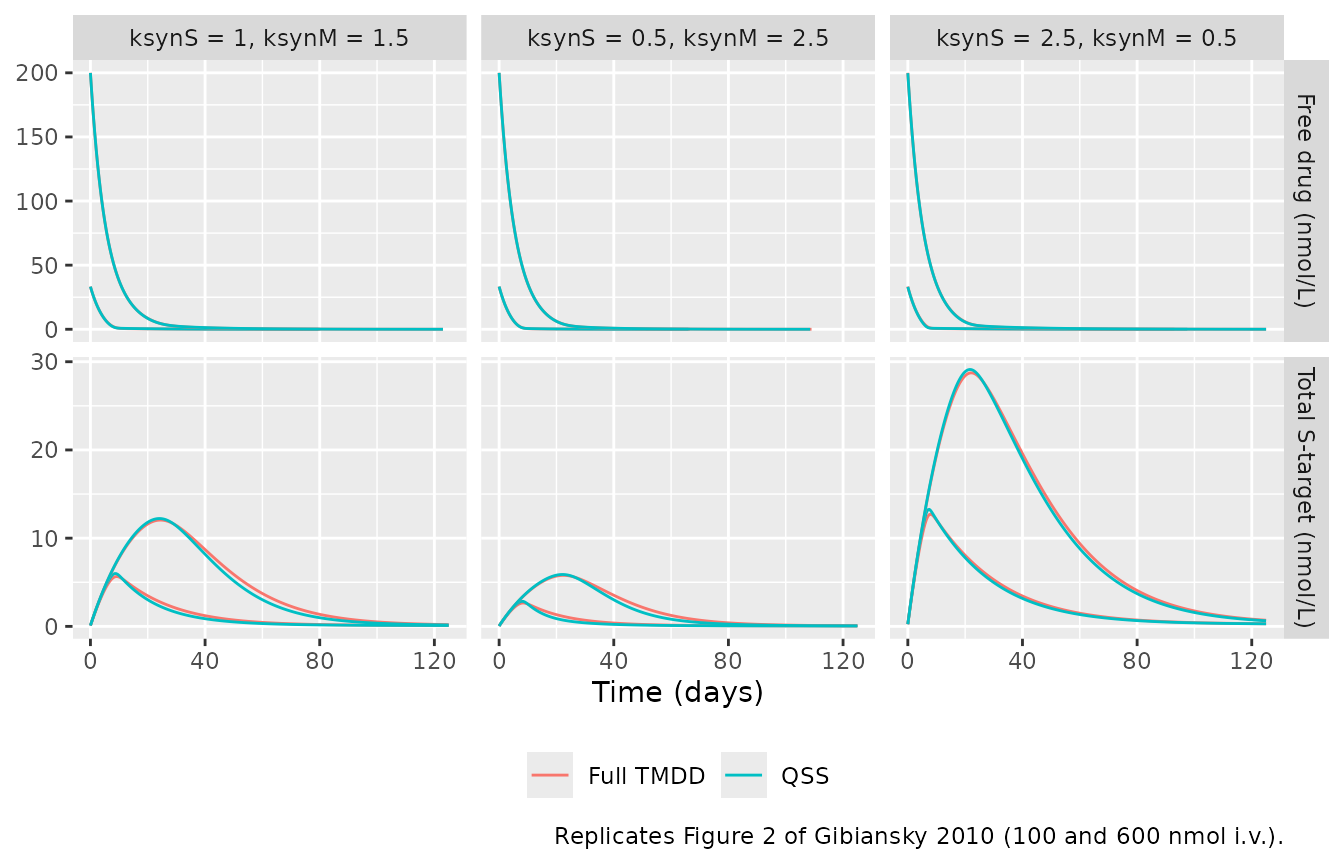
The free-drug rows of Figure 2 are on a log scale:
fig2 |>
  dplyr::filter(Cc >= 0.01, time <= 125) |>
  ggplot(aes(time, Cc, colour = model, group = interaction(model, dose))) +
  geom_line() +
  facet_wrap(~scenario) +
  scale_y_log10() +
  labs(x = "Time (days)", y = "Free drug (nmol/L)", colour = NULL,
       caption = "Replicates the top row of Figure 2 of Gibiansky 2010.") +
  theme(legend.position = "bottom")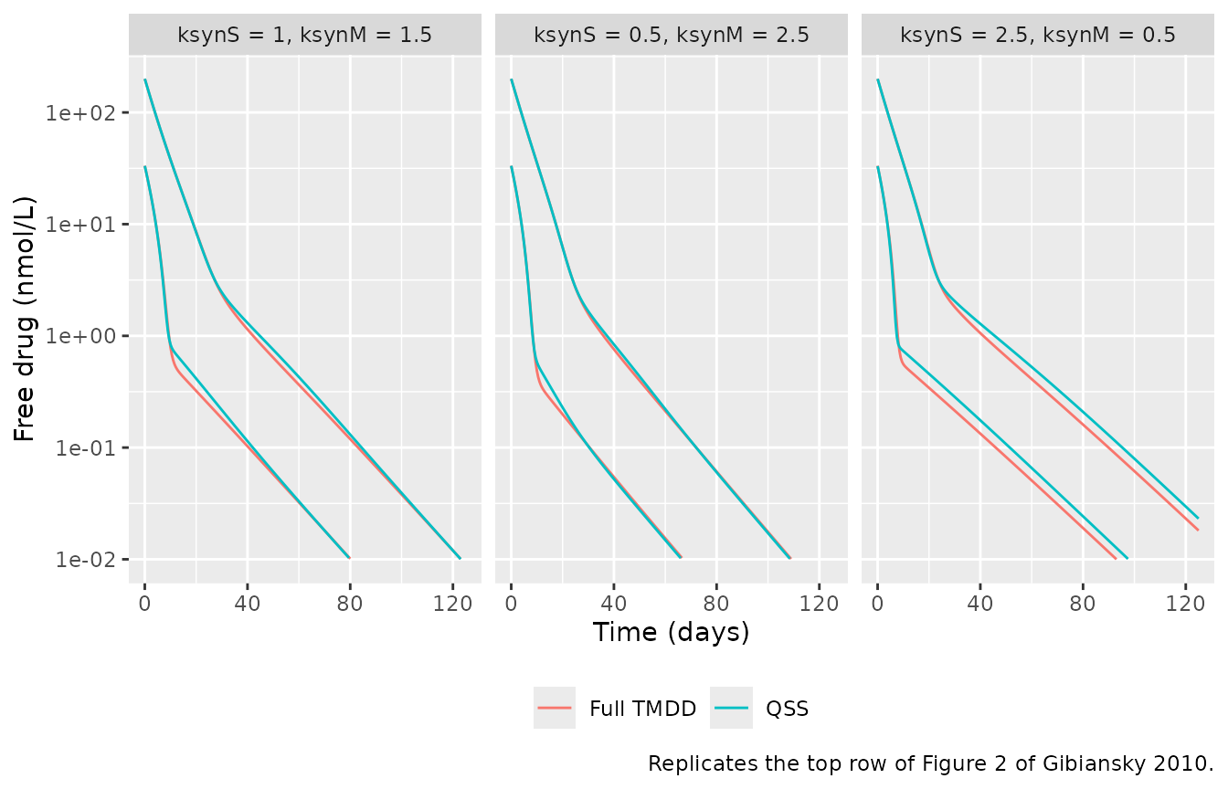
The total S-target peaks below were read off Figure 2 by the maintainers (about 12, 6 and 29 nmol/L at 600 nmol, and about 5.5, 2.5 and 13 nmol/L at 100 nmol), and are compared with both models.
peaks <- fig2 |>
  dplyr::group_by(scenario, dose, model) |>
  dplyr::summarise(peak = max(Ctotal_target_soluble), tpeak = time[which.max(Ctotal_target_soluble)],
                   .groups = "drop") |>
  tidyr::pivot_wider(names_from = model, values_from = c(peak, tpeak)) |>
  dplyr::left_join(
    tibble::tibble(
      scenario = rep(levels(scen$scenario), each = 2),
      dose = rep(c(100, 600), 3),
      digitised = c(5.5, 12, 2.5, 6, 13, 29)
    ) |>
      dplyr::mutate(scenario = factor(scenario, levels = levels(scen$scenario))),
    by = c("scenario", "dose")
  )
peaks |>
  dplyr::rename(
    Scenario = scenario, `Dose (nmol)` = dose,
    `Peak, full (nmol/L)` = `peak_Full TMDD`, `Peak, QSS (nmol/L)` = peak_QSS,
    `Day of peak, full` = `tpeak_Full TMDD`, `Day of peak, QSS` = tpeak_QSS,
    `Figure 2 (digitised)` = digitised
  ) |>
knitr::kable(digits = 2)| Scenario | Dose (nmol) | Peak, full (nmol/L) | Peak, QSS (nmol/L) | Day of peak, full | Day of peak, QSS | Figure 2 (digitised) |
|---|---|---|---|---|---|---|
| ksynS = 1, ksynM = 1.5 | 100 | 5.65 | 5.99 | 9.0 | 8.5 | 5.5 |
| ksynS = 1, ksynM = 1.5 | 600 | 12.05 | 12.23 | 24.5 | 24.0 | 12.0 |
| ksynS = 0.5, ksynM = 2.5 | 100 | 2.65 | 2.85 | 8.5 | 8.0 | 2.5 |
| ksynS = 0.5, ksynM = 2.5 | 600 | 5.79 | 5.88 | 22.5 | 22.0 | 6.0 |
| ksynS = 2.5, ksynM = 0.5 | 100 | 12.72 | 13.27 | 8.0 | 7.5 | 13.0 |
| ksynS = 2.5, ksynM = 0.5 | 600 | 28.74 | 29.12 | 22.0 | 21.5 | 29.0 |
conc_agree <- fig2 |>
  dplyr::select(scenario, dose, model, time, Cc) |>
  tidyr::pivot_wider(names_from = model, values_from = Cc) |>
  dplyr::filter(`Full TMDD` >= 0.01) |>
  dplyr::group_by(scenario, dose) |>
  dplyr::summarise(median_abs_log_ratio = median(abs(log(QSS / `Full TMDD`))), .groups = "drop")
knitr::kable(conc_agree, digits = 3,
caption = "Median |log(QSS / full)| of free drug while above 0.01 nmol/L.")| scenario | dose | median_abs_log_ratio |
|---|---|---|
| ksynS = 1, ksynM = 1.5 | 100 | 0.044 |
| ksynS = 1, ksynM = 1.5 | 600 | 0.040 |
| ksynS = 0.5, ksynM = 2.5 | 100 | 0.039 |
| ksynS = 0.5, ksynM = 2.5 | 600 | 0.021 |
| ksynS = 2.5, ksynM = 0.5 | 100 | 0.256 |
| ksynS = 2.5, ksynM = 0.5 | 600 | 0.245 |
stopifnot(
  # Both models land on the figure's peaks; a mis-transcribed ksyn, kdeg or
  # kint moves these by tens of percent.
  all(abs(peaks$`peak_Full TMDD` / peaks$digitised - 1) < 0.15),
  all(abs(peaks$peak_QSS / peaks$digitised - 1) < 0.15),
  # The approximation tracks the full model's total target closely.
  all(abs(peaks$peak_QSS / peaks$`peak_Full TMDD` - 1) < 0.10),
  # Free drug: about 2-4% when the M-target contributes (measured 0.021-0.044)
  # and about 25% when the S-target dominates (0.24-0.26), where Figure 2 also
  # shows the QSS line visibly above the full model late in the profile.
  all(conc_agree$median_abs_log_ratio[conc_agree$scenario != "ksynS = 2.5, ksynM = 0.5"] < 0.08),
  all(conc_agree$median_abs_log_ratio < 0.35)
)
Figure 3: contributions of the two elimination routes
The full model is solved with only linear elimination (both target syntheses switched off), linear + S-target, linear + M-target, and all three routes, after 100 nmol i.v. and 1000 nmol s.c.
off <- 1e-12
routes <- tibble::tibble(
  route = c("Only linear", "Only S-target", "Only M-target", "Both routes"),
  s_on = c(FALSE, TRUE, FALSE, TRUE),
  m_on = c(FALSE, FALSE, TRUE, TRUE)
)
fig3 <- tidyr::expand_grid(scen, routes,
  regimen = c("100 nmol i.v.", "1000 nmol s.c.")) |>
  dplyr::rowwise() |>
  dplyr::mutate(sim = list(
    solve_typical(
      mod_full,
      make_events(1L, 0,
                  if (regimen == "100 nmol i.v.") 100 else 1000,
                  if (regimen == "100 nmol i.v.") "central" else "depot", grid),
      params_full(if (s_on) ksyn_s else off, if (m_on) ksyn_m else off)
    ) |>
      dplyr::select(time, Cc)
  )) |>
  dplyr::ungroup() |>
  tidyr::unnest(sim) |>
  dplyr::mutate(route = factor(route, levels = routes$route))
#> ℹ parameter labels from comments will be replaced by 'label()'
#> ℹ omega/sigma items treated as zero: 'etalcl', 'etalvc', 'etalq', 'etalvp', 'etalka', 'etalkint_s', 'etalksyn_s', 'etalkdeg_s', 'etalkint_m', 'etalksyn_m', 'etalkdeg_m'
#> ℹ parameter labels from comments will be replaced by 'label()'
#> ℹ omega/sigma items treated as zero: 'etalcl', 'etalvc', 'etalq', 'etalvp', 'etalka', 'etalkint_s', 'etalksyn_s', 'etalkdeg_s', 'etalkint_m', 'etalksyn_m', 'etalkdeg_m'
#> ℹ parameter labels from comments will be replaced by 'label()'
#> ℹ omega/sigma items treated as zero: 'etalcl', 'etalvc', 'etalq', 'etalvp', 'etalka', 'etalkint_s', 'etalksyn_s', 'etalkdeg_s', 'etalkint_m', 'etalksyn_m', 'etalkdeg_m'
#> ℹ parameter labels from comments will be replaced by 'label()'
#> ℹ omega/sigma items treated as zero: 'etalcl', 'etalvc', 'etalq', 'etalvp', 'etalka', 'etalkint_s', 'etalksyn_s', 'etalkdeg_s', 'etalkint_m', 'etalksyn_m', 'etalkdeg_m'
#> ℹ parameter labels from comments will be replaced by 'label()'
#> ℹ omega/sigma items treated as zero: 'etalcl', 'etalvc', 'etalq', 'etalvp', 'etalka', 'etalkint_s', 'etalksyn_s', 'etalkdeg_s', 'etalkint_m', 'etalksyn_m', 'etalkdeg_m'
#> ℹ parameter labels from comments will be replaced by 'label()'
#> ℹ omega/sigma items treated as zero: 'etalcl', 'etalvc', 'etalq', 'etalvp', 'etalka', 'etalkint_s', 'etalksyn_s', 'etalkdeg_s', 'etalkint_m', 'etalksyn_m', 'etalkdeg_m'
#> ℹ parameter labels from comments will be replaced by 'label()'
#> ℹ omega/sigma items treated as zero: 'etalcl', 'etalvc', 'etalq', 'etalvp', 'etalka', 'etalkint_s', 'etalksyn_s', 'etalkdeg_s', 'etalkint_m', 'etalksyn_m', 'etalkdeg_m'
#> ℹ parameter labels from comments will be replaced by 'label()'
#> ℹ omega/sigma items treated as zero: 'etalcl', 'etalvc', 'etalq', 'etalvp', 'etalka', 'etalkint_s', 'etalksyn_s', 'etalkdeg_s', 'etalkint_m', 'etalksyn_m', 'etalkdeg_m'
#> ℹ parameter labels from comments will be replaced by 'label()'
#> ℹ omega/sigma items treated as zero: 'etalcl', 'etalvc', 'etalq', 'etalvp', 'etalka', 'etalkint_s', 'etalksyn_s', 'etalkdeg_s', 'etalkint_m', 'etalksyn_m', 'etalkdeg_m'
#> ℹ parameter labels from comments will be replaced by 'label()'
#> ℹ omega/sigma items treated as zero: 'etalcl', 'etalvc', 'etalq', 'etalvp', 'etalka', 'etalkint_s', 'etalksyn_s', 'etalkdeg_s', 'etalkint_m', 'etalksyn_m', 'etalkdeg_m'
#> ℹ parameter labels from comments will be replaced by 'label()'
#> ℹ omega/sigma items treated as zero: 'etalcl', 'etalvc', 'etalq', 'etalvp', 'etalka', 'etalkint_s', 'etalksyn_s', 'etalkdeg_s', 'etalkint_m', 'etalksyn_m', 'etalkdeg_m'
#> ℹ parameter labels from comments will be replaced by 'label()'
#> ℹ omega/sigma items treated as zero: 'etalcl', 'etalvc', 'etalq', 'etalvp', 'etalka', 'etalkint_s', 'etalksyn_s', 'etalkdeg_s', 'etalkint_m', 'etalksyn_m', 'etalkdeg_m'
#> ℹ parameter labels from comments will be replaced by 'label()'
#> ℹ omega/sigma items treated as zero: 'etalcl', 'etalvc', 'etalq', 'etalvp', 'etalka', 'etalkint_s', 'etalksyn_s', 'etalkdeg_s', 'etalkint_m', 'etalksyn_m', 'etalkdeg_m'
#> ℹ parameter labels from comments will be replaced by 'label()'
#> ℹ omega/sigma items treated as zero: 'etalcl', 'etalvc', 'etalq', 'etalvp', 'etalka', 'etalkint_s', 'etalksyn_s', 'etalkdeg_s', 'etalkint_m', 'etalksyn_m', 'etalkdeg_m'
#> ℹ parameter labels from comments will be replaced by 'label()'
#> ℹ omega/sigma items treated as zero: 'etalcl', 'etalvc', 'etalq', 'etalvp', 'etalka', 'etalkint_s', 'etalksyn_s', 'etalkdeg_s', 'etalkint_m', 'etalksyn_m', 'etalkdeg_m'
#> ℹ parameter labels from comments will be replaced by 'label()'
#> ℹ omega/sigma items treated as zero: 'etalcl', 'etalvc', 'etalq', 'etalvp', 'etalka', 'etalkint_s', 'etalksyn_s', 'etalkdeg_s', 'etalkint_m', 'etalksyn_m', 'etalkdeg_m'
#> ℹ parameter labels from comments will be replaced by 'label()'
#> ℹ omega/sigma items treated as zero: 'etalcl', 'etalvc', 'etalq', 'etalvp', 'etalka', 'etalkint_s', 'etalksyn_s', 'etalkdeg_s', 'etalkint_m', 'etalksyn_m', 'etalkdeg_m'
#> ℹ parameter labels from comments will be replaced by 'label()'
#> ℹ omega/sigma items treated as zero: 'etalcl', 'etalvc', 'etalq', 'etalvp', 'etalka', 'etalkint_s', 'etalksyn_s', 'etalkdeg_s', 'etalkint_m', 'etalksyn_m', 'etalkdeg_m'
#> ℹ parameter labels from comments will be replaced by 'label()'
#> ℹ omega/sigma items treated as zero: 'etalcl', 'etalvc', 'etalq', 'etalvp', 'etalka', 'etalkint_s', 'etalksyn_s', 'etalkdeg_s', 'etalkint_m', 'etalksyn_m', 'etalkdeg_m'
#> ℹ parameter labels from comments will be replaced by 'label()'
#> ℹ omega/sigma items treated as zero: 'etalcl', 'etalvc', 'etalq', 'etalvp', 'etalka', 'etalkint_s', 'etalksyn_s', 'etalkdeg_s', 'etalkint_m', 'etalksyn_m', 'etalkdeg_m'
#> ℹ parameter labels from comments will be replaced by 'label()'
#> ℹ omega/sigma items treated as zero: 'etalcl', 'etalvc', 'etalq', 'etalvp', 'etalka', 'etalkint_s', 'etalksyn_s', 'etalkdeg_s', 'etalkint_m', 'etalksyn_m', 'etalkdeg_m'
#> ℹ parameter labels from comments will be replaced by 'label()'
#> ℹ omega/sigma items treated as zero: 'etalcl', 'etalvc', 'etalq', 'etalvp', 'etalka', 'etalkint_s', 'etalksyn_s', 'etalkdeg_s', 'etalkint_m', 'etalksyn_m', 'etalkdeg_m'
#> ℹ parameter labels from comments will be replaced by 'label()'
#> ℹ omega/sigma items treated as zero: 'etalcl', 'etalvc', 'etalq', 'etalvp', 'etalka', 'etalkint_s', 'etalksyn_s', 'etalkdeg_s', 'etalkint_m', 'etalksyn_m', 'etalkdeg_m'
#> ℹ parameter labels from comments will be replaced by 'label()'
#> ℹ omega/sigma items treated as zero: 'etalcl', 'etalvc', 'etalq', 'etalvp', 'etalka', 'etalkint_s', 'etalksyn_s', 'etalkdeg_s', 'etalkint_m', 'etalksyn_m', 'etalkdeg_m'

fig3 |>
  dplyr::filter(Cc >= 0.01, time <= 125) |>
  ggplot(aes(time, Cc, colour = route)) +
  geom_line() +
  facet_grid(regimen ~ scenario) +
  scale_y_log10() +
  labs(x = "Time (days)", y = "Free drug (nmol/L)", colour = NULL,
       caption = "Replicates Figure 3 of Gibiansky 2010.") +
  theme(legend.position = "bottom")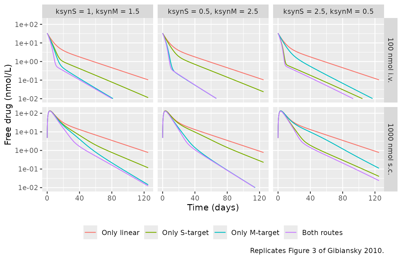
c60 <- fig3 |>
  dplyr::filter(time == 60) |>
  dplyr::select(scenario, regimen, route, Cc) |>
  tidyr::pivot_wider(names_from = route, values_from = Cc)
knitr::kable(c60, digits = 4, caption = "Free drug (nmol/L) on day 60.")| scenario | regimen | Only linear | Only S-target | Only M-target | Both routes |
|---|---|---|---|---|---|
| ksynS = 1, ksynM = 1.5 | 100 nmol i.v. | 0.9024 | 0.1809 | 0.0364 | 0.0323 |
| ksynS = 1, ksynM = 1.5 | 1000 nmol s.c. | 6.7687 | 1.9664 | 0.8101 | 0.4983 |
| ksynS = 0.5, ksynM = 2.5 | 100 nmol i.v. | 0.9024 | 0.3174 | 0.0154 | 0.0154 |
| ksynS = 0.5, ksynM = 2.5 | 1000 nmol s.c. | 6.7687 | 3.7003 | 0.3182 | 0.2949 |
| ksynS = 2.5, ksynM = 0.5 | 100 nmol i.v. | 0.9024 | 0.0750 | 0.1890 | 0.0508 |
| ksynS = 2.5, ksynM = 0.5 | 1000 nmol s.c. | 6.7687 | 0.7194 | 3.6310 | 0.5368 |
Figure 3’s message is that whichever target has the five-fold higher synthesis rate dominates target-mediated elimination: when ksynS = 0.5 and ksynM = 2.5 the “Only M-target” curve lies close to “Both routes”, and when ksynS = 2.5 and ksynM = 0.5 the “Only S-target” curve does.
gap <- function(sc, r) {
  row <- c60[c60$scenario == sc & c60$regimen == "100 nmol i.v.", ]
  abs(log(row[[r]] / row[["Both routes"]]))
}
stopifnot(
  # Every route removes drug: on day 60 each target-mediated route sits at
  # least two-fold below linear-only (deterministic; smallest measured 12.6x).
  all(c60[["Only linear"]] > 2 * c60[["Both routes"]]),
  all(c60[["Only linear"]] > c60[["Only S-target"]]),
  all(c60[["Only linear"]] > c60[["Only M-target"]]),
  # The dominant target is the one closer to the complete system.
  gap("ksynS = 0.5, ksynM = 2.5", "Only M-target") < gap("ksynS = 0.5, ksynM = 2.5", "Only S-target"),
  gap("ksynS = 2.5, ksynM = 0.5", "Only S-target") < gap("ksynS = 2.5, ksynM = 0.5", "Only M-target")
)
Membrane-target suppression (Figure 6)
The paper derives the unobservable percent decrease of free M-target
from baseline from the QSS model as 100 * C / (C + KSS_M)
and compares it with the value simulated from the full model,
100 * (R0_M - R_M) / R0_M. It notes that the QSS
approximation over-predicts the decrease 1 hour after an s.c. dose.
pd_grid <- sort(unique(c(1 / 24, grid[grid > 0])))
fig6 <- tibble::tibble(regimen = c("600 nmol i.v.", "1000 nmol s.c.")) |>
  dplyr::rowwise() |>
  dplyr::mutate(sim = list({
    ev <- make_events(1L, 0, if (regimen == "600 nmol i.v.") 600 else 1000,
                      if (regimen == "600 nmol i.v.") "central" else "depot", pd_grid)
    f <- solve_typical(mod_full, ev)
    q <- solve_typical(mod_qss, ev)
    tibble::tibble(
      time = f$time,
      full = 100 * (0.1 - f$target_membrane) / 0.1,
      qss = 100 * q$Cc / (q$Cc + 3.05)
    )
  })) |>
  dplyr::ungroup() |>
  tidyr::unnest(sim)
#> ℹ parameter labels from comments will be replaced by 'label()'
#> ℹ omega/sigma items treated as zero: 'etalcl', 'etalvc', 'etalq', 'etalvp', 'etalka', 'etalkint_s', 'etalksyn_s', 'etalkdeg_s', 'etalkint_m', 'etalksyn_m', 'etalkdeg_m'
#> ℹ parameter labels from comments will be replaced by 'label()'
#> ℹ omega/sigma items treated as zero: 'etalcl', 'etalvc', 'etalq', 'etalvp', 'etalka', 'etalkint_s', 'etalkdeg_s'
#> ℹ parameter labels from comments will be replaced by 'label()'
#> ℹ omega/sigma items treated as zero: 'etalcl', 'etalvc', 'etalq', 'etalvp', 'etalka', 'etalkint_s', 'etalksyn_s', 'etalkdeg_s', 'etalkint_m', 'etalksyn_m', 'etalkdeg_m'
#> ℹ parameter labels from comments will be replaced by 'label()'
#> ℹ omega/sigma items treated as zero: 'etalcl', 'etalvc', 'etalq', 'etalvp', 'etalka', 'etalkint_s', 'etalkdeg_s'

fig6 |>
  tidyr::pivot_longer(c(full, qss), names_to = "model", values_to = "pct") |>
  dplyr::filter(time <= 125) |>
  ggplot(aes(time, pct, colour = model)) +
  geom_line() +
  facet_wrap(~regimen) +
  labs(x = "Time (days)", y = "Free M-target decrease from baseline (%)", colour = NULL,
       caption = "Typical-value analogue of Figure 6 of Gibiansky 2010.") +
  theme(legend.position = "bottom")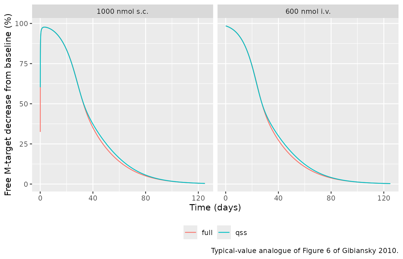
m_err <- fig6 |>
  dplyr::mutate(early = time < 1) |>
  dplyr::group_by(regimen, early) |>
  dplyr::summarise(max_abs_diff = max(abs(full - qss)), .groups = "drop")
knitr::kable(m_err, digits = 2, caption = "Largest absolute difference (percentage points).")| regimen | early | max_abs_diff |
|---|---|---|
| 1000 nmol s.c. | FALSE | 2.79 |
| 1000 nmol s.c. | TRUE | 27.83 |
| 600 nmol i.v. | FALSE | 2.72 |
| 600 nmol i.v. | TRUE | 0.00 |
sc_1h <- fig6 |> dplyr::filter(regimen == "1000 nmol s.c.", abs(time - 1 / 24) < 1e-9)
stopifnot(
  # From day 1 on, the QSS prediction of the unobserved M-target suppression
  # tracks the full model to within a few percentage points.
  all(m_err$max_abs_diff[!m_err$early] < 5),
  # At 1 h after the s.c. dose the QSS over-predicts it, as the paper reports.
  nrow(sc_1h) == 1L,
  sc_1h$qss > sc_1h$full
)
Simulated studies (Table 2)
The two studies of Table 2 are simulated from the full model with the assumed variability. Study 2’s sampling list in Table 2 reads “1, 24 h; then 1, 7, 14, 28 (pre-dose), 56 (pre-dose), 63, …, 112 days”; it is used as printed, so day 1 is sampled twice. That gives 13 samples per Study 1 subject and 15 per Study 2 subject, or 3,312 per output before the 0.1 nmol/L quantification limit is applied, which agrees with the paper’s 3,298 drug and 3,257 S-target observations remaining after it. Pre-dose samples are placed one minute before the dose.
rxode2::rxSetSeed(20100729)
t1 <- c(1, 6, 12, 24) / 24
t1 <- c(t1, 3, 7, 14, 21, 28, 35, 42, 49, 56)
pre <- 1 / 1440
t2 <- c(1 / 24, 1, 1, 7, 14, 28 - pre, 56 - pre, 63, 70, 77, 84, 91, 98, 105, 112)

arms <- tibble::tribble(
  ~treatment,                  ~n,  ~amt, ~cmt,      ~study,
  "Study 1: 100 nmol i.v.",    6L,  100,  "central", 1L,
  "Study 1: 300 nmol i.v.",    6L,  300,  "central", 1L,
  "Study 1: 600 nmol i.v.",    6L,  600,  "central", 1L,
  "Study 1: 1000 nmol s.c.",   6L,  1000, "depot",   1L,
  "Study 2: 600 nmol i.v. x3", 100L, 600, "central", 2L,
  "Study 2: 1000 nmol s.c. x3", 100L, 1000, "depot", 2L
) |>
  dplyr::mutate(id_offset = cumsum(dplyr::lag(n, default = 0L)))

events <- arms |>
  dplyr::rowwise() |>
  dplyr::mutate(ev = list(make_events(
    ids = id_offset + seq_len(n),
    dose_times = if (study == 1L) 0 else c(0, 28, 56),
    amt = amt, cmt = cmt,
    times = if (study == 1L) t1 else t2,
    dvid = c(1L, 2L)
  ))) |>
  dplyr::ungroup() |>
  dplyr::select(treatment, ev) |>
  tidyr::unnest(ev) |>
  as.data.frame()
stopifnot(
  length(unique(events$id)) == 224L,
  !anyDuplicated(unique(events[events$evid == 1L, c("id", "time")]))
)
sim <- rxode2::rxSolve(mod_full, events = events, keep = "treatment",
                       returnType = "data.frame")
#> ℹ parameter labels from comments will be replaced by 'label()'
# The endpoint of each observation row is its CMT: the first `~` endpoint (Cc)
# takes the lower number. Confirm that before using it.
obs <- sim |>
  dplyr::mutate(output = ifelse(CMT == min(CMT), "Free drug", "Total S-target"))
stopifnot(
  isTRUE(all.equal(obs$ipredSim[obs$output == "Free drug"], obs$Cc[obs$output == "Free drug"])),
  isTRUE(all.equal(obs$ipredSim[obs$output == "Total S-target"],
                   obs$Ctotal_target_soluble[obs$output == "Total S-target"]))
)
counts <- obs |>
  dplyr::group_by(output) |>
  dplyr::summarise(records = dplyr::n(), above_LOQ = sum(sim >= 0.1), .groups = "drop") |>
  dplyr::mutate(paper = c(3298L, 3257L))
knitr::kable(counts, caption = "Observation records before and after removing values below 0.1 nmol/L.")| output | records | above_LOQ | paper |
|---|---|---|---|
| Free drug | 3312 | 3292 | 3298 |
| Total S-target | 3312 | 3251 | 3257 |
stopifnot(
  all(counts$records == 3312L),
  # The paper removed 14 drug and 55 S-target records (0.4% and 1.7%); the
  # number below the limit depends on the cohort drawn, so the gate is on the
  # retained fraction, not the count. A ten-fold error in a baseline or a
  # volume would push many more records below 0.1 nmol/L.
  all(counts$above_LOQ / counts$records > 0.95)
)
The number of simulated records left above 0.1 nmol/L lands close to the paper’s counts (the exact number depends on the cohort drawn), which is an end-to-end check of the baselines, the variability and the dosing design together.
obs |>
  dplyr::filter(sim >= 0.1, grepl("Study 2", treatment)) |>
  dplyr::mutate(time_bin = round(time)) |>
  dplyr::group_by(treatment, output, time_bin) |>
  dplyr::summarise(
    Q05 = quantile(sim, 0.05), Q50 = quantile(sim, 0.50), Q95 = quantile(sim, 0.95),
    .groups = "drop"
  ) |>
  ggplot(aes(time_bin, Q50)) +
  geom_ribbon(aes(ymin = Q05, ymax = Q95), alpha = 0.25) +
  geom_line() +
  facet_grid(output ~ treatment, scales = "free_y") +
  scale_y_log10() +
  labs(x = "Time (days)", y = "Concentration (nmol/L)",
       caption = "Simulated Study 2 (Table 2): median and 90% interval, values below 0.1 nmol/L removed.")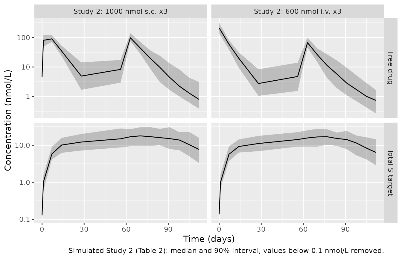
PKNCA validation
The paper reports no NCA. Non-compartmental analysis of the typical-value free-drug profile for each single-dose arm of Study 1 shows the TMDD signature: dose-normalised exposure rises with the i.v. dose as the targets saturate.
nca_grid <- sort(unique(c(seq(0, 1, by = 1 / 24), seq(1, 365, by = 0.5))))
single <- arms |> dplyr::filter(study == 1L)
sim_nca <- single |>
  dplyr::rowwise() |>
  dplyr::mutate(sim = list(
    solve_typical(mod_full, make_events(1L, 0, amt, cmt, nca_grid)) |>
      dplyr::select(time, Cc)
  )) |>
  dplyr::ungroup() |>
  dplyr::mutate(id = dplyr::row_number()) |>
  dplyr::select(id, treatment, amt, sim) |>
  tidyr::unnest(sim)
#> ℹ parameter labels from comments will be replaced by 'label()'
#> ℹ omega/sigma items treated as zero: 'etalcl', 'etalvc', 'etalq', 'etalvp', 'etalka', 'etalkint_s', 'etalksyn_s', 'etalkdeg_s', 'etalkint_m', 'etalksyn_m', 'etalkdeg_m'
#> ℹ parameter labels from comments will be replaced by 'label()'
#> ℹ omega/sigma items treated as zero: 'etalcl', 'etalvc', 'etalq', 'etalvp', 'etalka', 'etalkint_s', 'etalksyn_s', 'etalkdeg_s', 'etalkint_m', 'etalksyn_m', 'etalkdeg_m'
#> ℹ parameter labels from comments will be replaced by 'label()'
#> ℹ omega/sigma items treated as zero: 'etalcl', 'etalvc', 'etalq', 'etalvp', 'etalka', 'etalkint_s', 'etalksyn_s', 'etalkdeg_s', 'etalkint_m', 'etalksyn_m', 'etalkdeg_m'
#> ℹ parameter labels from comments will be replaced by 'label()'
#> ℹ omega/sigma items treated as zero: 'etalcl', 'etalvc', 'etalq', 'etalvp', 'etalka', 'etalkint_s', 'etalksyn_s', 'etalkdeg_s', 'etalkint_m', 'etalksyn_m', 'etalkdeg_m'

stopifnot(all(sim_nca$Cc >= -1e-6 * max(sim_nca$Cc)))
conc_df <- sim_nca |>
  dplyr::filter(!is.na(Cc)) |>
  dplyr::mutate(Cc = pmax(Cc, 0)) |>
  dplyr::select(id, treatment, time, Cc)
conc_df <- dplyr::bind_rows(
  conc_df,
  conc_df |> dplyr::distinct(id, treatment) |> dplyr::mutate(time = 0, Cc = 0)
) |>
  dplyr::distinct(id, treatment, time, .keep_all = TRUE) |>
  dplyr::arrange(id, treatment, time)

dose_df <- sim_nca |>
  dplyr::distinct(id, treatment, amt) |>
  dplyr::mutate(time = 0, route = ifelse(grepl("s.c.", treatment), "extravascular", "intravascular"))

conc_obj <- PKNCA::PKNCAconc(conc_df, Cc ~ time | treatment + id)
dose_obj <- PKNCA::PKNCAdose(dose_df, amt ~ time | treatment + id, route = "route")
intervals <- data.frame(start = 0, end = Inf, cmax = TRUE, tmax = TRUE,
                        aucinf.obs = TRUE, half.life = TRUE)
nca_res <- PKNCA::pk.nca(PKNCA::PKNCAdata(conc_obj, dose_obj, intervals = intervals))

nca_tab <- as.data.frame(nca_res$result) |>
  dplyr::filter(PPTESTCD %in% c("cmax", "tmax", "aucinf.obs", "half.life")) |>
  dplyr::select(treatment, PPTESTCD, PPORRES) |>
  tidyr::pivot_wider(names_from = PPTESTCD, values_from = PPORRES) |>
  dplyr::left_join(dplyr::distinct(sim_nca, treatment, amt), by = "treatment") |>
  dplyr::mutate(auc_per_dose = aucinf.obs / amt)
nca_tab |>
  dplyr::rename(
    Arm = treatment, `Cmax (nmol/L)` = cmax, `Tmax (day)` = tmax,
    `AUCinf (nmol*day/L)` = aucinf.obs, `Terminal t1/2 (day)` = half.life,
    `Dose (nmol)` = amt, `AUCinf/dose (day/L)` = auc_per_dose
  ) |>
knitr::kable(digits = 3)| Arm | Cmax (nmol/L) | Tmax (day) | Terminal t1/2 (day) | AUCinf (nmol*day/L) | Dose (nmol) | AUCinf/dose (day/L) |
|---|---|---|---|---|---|---|
| Study 1: 100 nmol i.v. | 33.333 | 0.0 | 11.937 | 118.851 | 100 | 1.189 |
| Study 1: 1000 nmol s.c. | 129.688 | 3.5 | 11.949 | 1450.177 | 1000 | 1.450 |
| Study 1: 300 nmol i.v. | 100.000 | 0.0 | 11.966 | 513.633 | 300 | 1.712 |
| Study 1: 600 nmol i.v. | 200.000 | 0.0 | 11.955 | 1232.069 | 600 | 2.053 |
iv <- nca_tab |> dplyr::filter(grepl("i.v.", treatment)) |> dplyr::arrange(amt)
stopifnot(
  nrow(iv) == 3L,
  # Target-mediated clearance saturates: AUC/dose rises with the i.v. dose and
  # stays below the linear-only value Dose/CL, i.e. 1/0.3 day/L.
  iv$auc_per_dose[3] > iv$auc_per_dose[1],
  all(iv$auc_per_dose < 1 / 0.3),
  # The paper chose the linear part to give "the effective half-life of about
  # 10 days at high doses" (Identifiability section). The terminal phase here
  # is about 12 days in every arm (typical values, deterministic), against
  # 20.8 days for the linear part alone, because the targets keep removing
  # drug at low concentrations.
  all(nca_tab$half.life > 8 & nca_tab$half.life < 15)
)
The terminal half-life of about 12 days in every arm agrees with the paper’s design statement of “the effective half-life of about 10 days at high doses”. The paper reports no other NCA quantity, so there is no published table to compare against.
Assumptions and deviations
-
Methodology paper. No drug is named and every
dataset in the paper is simulated. The Table 1 values are the authors’
own nominal choices for a hypothetical fully human antibody, so every
ini()value is wrapped infixed(). The models are filed underpharmacokinetics/with a structural descriptor in place of a drug name. - Units of CL and Q. Table 1 prints the unit of CL and Q as “day^-1”; they are clearances in L/day, as the table’s own footnote (kel = CL/Vc, kpt = Q/Vc, ktp = Q/Vp) requires.
- Inter-individual variability. “Log-normal distributions with 20% CV” is encoded as omega^2 = log(1 + 0.2^2) = 0.0392; the alternative reading omega^2 = 0.2^2 = 0.04 differs by 2%. No correlation is stated, so none is assumed. The residual errors use the same convention (log-scale SD sqrt(log(1 + CV^2))).
- IIV on the QSS model. The paper does not report the random-effect estimates of the fitted QSS model M3. The QSS file carries the simulation’s 20% CV on the M3 parameters that are themselves simulation parameters (CL, Vc, Q, Vp, ka, kint_S, kdeg_S). R0_S, KSS_S, Vmax_M and KSS_M are composites of several simulation parameters and carry no IIV.
- QSS parameter values. The QSS file uses the TRUE values (Table 1, also the “True value” column of Table 5), not the M3 estimates fitted to the simulated data (Table 4), which were within 16% of truth except KSS_S (0.0107 vs 0.015).
- Figure 2 dose. The Results text describes Figure 2 as 100 and 1000 nmol boluses, the caption as 100 and 600 nmol. The 600 nmol reading is used; it matches the plotted initial concentration of about 200 nmol/L.
- Figure 2 peaks were digitised by the maintainers to about one significant figure; the gate allows 15%.
- Study 2 sampling. Day 1 appears twice in Table 2’s Study 2 sampling list (as “24 h” and as “1”). It is used as printed, because only that reading reproduces the 3,312 records per output implied by the paper’s observation counts.
- Elimination routes in Figure 3 are switched off by setting the corresponding target synthesis rate to 1e-12 nmol/L/day, which removes the target (and its route) without changing any other parameter.
- Errata. No correction notice was found for this article (Europe PMC and publisher search, 2026-10-17).