TMDD with two targets and with FcRn recycling (Dua 2015)
Source:vignettes/articles/Dua_2015_tmdd_tutorial.Rmd
Dua_2015_tmdd_tutorial.RmdModel and source
- Article: Dua P, Hawkins E, van der Graaf PH. A Tutorial on Target-Mediated Drug Disposition (TMDD) Models. CPT Pharmacometrics Syst Pharmacol. 2015;4(6):324-337. https://doi.org/10.1002/psp4.41 (PMC4505827, open access).
- Supplement: “Berkeley Madonna TMDD model library”, a Word document holding the authors’ runnable Berkeley Madonna code for eight TMDD models, each with a complete illustrative parameter set.
Dua 2015 is a tutorial. Its body walks through the TMDD model family, from the one-compartment Mager and Jusko model through the QE, QSS and Michaelis-Menten approximations to extensions for multiple targets, competing drugs, receptor-mediated endocytosis, FcRn recycling and binding outside the central compartment. It fits no data, and every structure in it is attributed to an earlier paper.
The library takes two of the eight supplement models, the two structures it did not already carry:
| Supplement model | Structure | In this library |
|---|---|---|
| 1 | One-compartment full TMDD | archetype PK_1cmt_tmdd_full
|
| 2 | Two-compartment full TMDD | structure covered by the archetypes |
| 3 | Two-compartment QE approximation | structure covered by the archetypes |
| 4 | Two-compartment QSS approximation | archetype PK_2cmt_tmdd_qss
|
| 5 | Two-compartment MM approximation | archetype PK_2cmt_tmdd_mm
|
| 6 | Two targets: soluble (QSS) + membrane (MM), after Gibiansky & Gibiansky 2010 | Dua_2015_tmdd_multitarget_qss |
| 7 | Full TMDD with FcRn endosomal recycling, after Xiao 2010 | Dua_2015_tmdd_fcrn_recycling |
| 8 | Two-compartment QSS with denosumab values from Gibiansky 2012 | not taken; the values belong to the Gibiansky 2012 denosumab analysis, which carries the variability and covariate model this transcription drops |
mods <- c("Dua_2015_tmdd_multitarget_qss", "Dua_2015_tmdd_fcrn_recycling")
m6 <- rxode2::rxode2(readModelDb(mods[1]))
m7 <- rxode2::rxode2(readModelDb(mods[2]))

tibble::tibble(
  Model = mods,
  `Supplement model` = c(6L, 7L),
  `ODE states` = c(length(m6$state), length(m7$state)),
  Parameters = c(nrow(m6$iniDf), nrow(m7$iniDf))
) |>
knitr::kable()| Model | Supplement model | ODE states | Parameters |
|---|---|---|---|
| Dua_2015_tmdd_multitarget_qss | 6 | 3 | 14 |
| Dua_2015_tmdd_fcrn_recycling | 7 | 9 | 15 |
Population
There is no population. Both parameter sets are illustrative values
for a generic monoclonal antibody, chosen by the authors for teaching.
They are not fitted to data, and the source has no inter-individual
variability and no residual error. Every ini() value is
therefore fixed(), and the residual error is
fixed(0) so the models simulate exactly as written.
pop <- readModelDb(mods[1])() |>
  environment() |>
  (\(e) e$population)()
tibble::tibble(Field = names(pop), Value = vapply(pop, \(x) paste(as.character(x), collapse = " "), "")) |>
knitr::kable()| Value |
|---|
Units and the dose conversion
Time is days and every concentration is nM.
-
Model 6 works per kg body weight. The supplement
doses 10 mg/kg and converts it with
Dose = (Dosemg * 1e-3 / MWlig) * 1e9nmol/kg usingMWlig = 150000Da, then setsLc0 = Dose / VcwithVc = 0.04L/kg. The model file is molar (dosing in nmol/kg), so the conversion is applied here. -
Model 7 has no volume. The supplement gives the
dose as the initial central concentration
Lc0 = 200nM, and every transfer between compartments is a symmetric first-order rate constant, so all nine states are concentrations referenced to the central volume. A dose ofamt = 200intocentralreproduces it.
MW <- 150000 # Supplement Model 6: MWlig = 150000 Da
VC <- 0.04 # Supplement Model 6: Vc = 0.04 L/kg
mgkg_to_nmolkg <- function(mgkg) mgkg * 1e-3 / MW * 1e9

dose6 <- mgkg_to_nmolkg(10)
tibble::tibble(
  Quantity = c("Model 6 dose (nmol/kg)", "Model 6 Lc0 = Dose/Vc (nM)", "Model 7 Lc0 (nM)"),
  Value = c(dose6, dose6 / VC, 200)
) |>
knitr::kable(digits = 2)| Quantity | Value |
|---|---|
| Model 6 dose (nmol/kg) | 66.67 |
| Model 6 Lc0 = Dose/Vc (nM) | 1666.67 |
| Model 7 Lc0 (nM) | 200.00 |
Source trace
Equations are the main text’s Eqs V.1-V.6 for Model 6. Model 7 is described only in prose in the main text (“FcRn recycling”), so its equations come from the supplement alone. All parameter values come from the supplement.
tibble::tribble(
  ~Model, ~Quantity, ~`Source location`,
  "6", "d/dt Ltot (central), d/dt LT (peripheral1)", "Eqs V.2-V.3; Supplement Model 6 Lctot', Lt'",
  "6", "d/dt Rtot_S (total_target)", "Eq V.4; Supplement Model 6 Rstot'",
  "6", "Free drug LC from the soluble-target QSS quadratic", "Eq V.5; Supplement Model 6 Lc",
  "6", "Rtot_S(0) = R0_S = kin_S/kout_S; LT(0) = 0", "Eq V.6; Supplement Model 6 INIT and kins",
  "6", "Kss_S, Kss_M, Vmax_M = R0_M * kint_M", "Main text 'Multiple targets'; Supplement Model 6",
  "6", "Soluble complex Ps and free soluble target Rs", "Supplement Model 6 'Finding Amount of Free Receptor'",
  "7", "d/dt Lc, Lt, R, Pc, Pt, Le, FcLe, Pe, FcPe", "Supplement Model 7 'Ordinary Differential Equations'",
  "7", "kin = kout * R0; R(0) = R0; all other states 0 except Lc(0) = Lc0", "Supplement Model 7 INIT and rate constants"
) |>
knitr::kable()| Model | Quantity | Source location |
|---|---|---|
| 6 | d/dt Ltot (central), d/dt LT (peripheral1) | Eqs V.2-V.3; Supplement Model 6 Lctot’, Lt’ |
| 6 | d/dt Rtot_S (total_target) | Eq V.4; Supplement Model 6 Rstot’ |
| 6 | Free drug LC from the soluble-target QSS quadratic | Eq V.5; Supplement Model 6 Lc |
| 6 | Rtot_S(0) = R0_S = kin_S/kout_S; LT(0) = 0 | Eq V.6; Supplement Model 6 INIT and kins |
| 6 | Kss_S, Kss_M, Vmax_M = R0_M * kint_M | Main text ‘Multiple targets’; Supplement Model 6 |
| 6 | Soluble complex Ps and free soluble target Rs | Supplement Model 6 ‘Finding Amount of Free Receptor’ |
| 7 | d/dt Lc, Lt, R, Pc, Pt, Le, FcLe, Pe, FcPe | Supplement Model 7 ‘Ordinary Differential Equations’ |
| 7 | kin = kout * R0; R(0) = R0; all other states 0 except Lc(0) = Lc0 | Supplement Model 7 INIT and rate constants |
trace_params <- function(ui) {
  ui$iniDf |>
    dplyr::filter(!is.na(ntheta)) |>
    dplyr::transmute(Parameter = name, Value = signif(ifelse(grepl("^l", name), exp(est), est), 4), Label = label)
}
knitr::kable(trace_params(m6), caption = "Model 6 parameters (all from Supplement Model 6)")| Parameter | Value | Label |
|---|---|---|
| lvc | 4.00e-02 | Central volume of distribution (L/kg) |
| lkel | 4.60e-02 | Linear elimination rate constant of free drug from central (1/day) |
| lk12 | 9.02e-01 | Central-to-tissue transfer rate constant of free drug (1/day) |
| lk21 | 7.25e-01 | Tissue-to-central transfer rate constant of free drug (1/day) |
| lrbase_total_target | 6.57e-03 | Baseline soluble target concentration Rs0 (nM) |
| lkdeg_sol | 1.73e+01 | First-order degradation rate constant of free soluble target (1/day) |
| lkint_sol | 1.70e-01 | Elimination rate constant of the drug-soluble-target complex (1/day) |
| lkon_sol | 3.02e+01 | Association rate constant, drug to soluble target (1/(nM*day)) |
| lkoff_sol | 1.69e+02 | Dissociation rate constant of the drug-soluble-target complex (1/day) |
| lrtot_mem | 2.00e-03 | Total membrane-target concentration, held constant Rm0 (nM) |
| lkint_mem | 1.70e-01 | Elimination rate constant of the drug-membrane-target complex (1/day) |
| lkon_mem | 3.02e+01 | Association rate constant, drug to membrane target (1/(nM*day)) |
| lkoff_mem | 1.69e+02 | Dissociation rate constant of the drug-membrane-target complex (1/day) |
| propSd | 0.00e+00 | Proportional residual error (fraction; ZERO - none in the source) |
knitr::kable(trace_params(m7), caption = "Model 7 parameters (all from Supplement Model 7)")| Parameter | Value | Label |
|---|---|---|
| lkel | 0.024 | Elimination rate constant of free drug from central (1/day) |
| lkel_endo | 0.024 | Elimination rate constant of non-FcRn-bound drug and complex from the endosome (1/day) |
| lk12 | 0.902 | Central-to-tissue transfer rate constant of drug and complex (1/day) |
| lk21 | 0.725 | Tissue-to-central transfer rate constant of drug and complex (1/day) |
| lkup | 0.360 | Central-to-endosome uptake rate constant of drug and complex (1/day) |
| lrbase_target | 0.030 | Baseline free target concentration R0 (nM) |
| lkdeg | 0.823 | First-order degradation rate constant of free target (1/day) |
| lkint | 0.201 | Elimination rate constant of the drug-target complex from central (1/day) |
| lkon | 0.592 | Association rate constant, drug to target (1/(nM*day)) |
| lkoff | 0.900 | Dissociation rate constant of the drug-target complex (1/day) |
| lrtot_fcrn | 0.050 | Endosomal FcRn concentration, held constant Fc0 (nM) |
| lkon_fcrn | 4.830 | Association rate constant, drug or complex to FcRn (1/(nM*day)) |
| lkoff_fcrn | 2.000 | Dissociation rate constant of the FcRn complexes (1/day) |
| lkrec_fcrn | 0.400 | Recycling rate constant of FcRn complexes back to central (1/day) |
| propSd | 0.000 | Proportional residual error (fraction; ZERO - none in the source) |
Every value in both tables appears verbatim in the supplement; the
in-file comment on each ini() line names the supplement
variable it came from (kpt is the library’s
k12, ktp its k21,
kout its kdeg, and kep its
kint).
Units of every ODE term
| Model | State | Units | Every term reduces to |
|---|---|---|---|
| 6 |
central (total drug amount) |
nmol/kg |
(L/kg) x (1/day) x nM = nmol/kg/day |
| 6 |
peripheral1 (tissue drug amount, = Lt x Vc) |
nmol/kg |
(1/day) x (L/kg) x nM or
(1/day) x nmol/kg
|
| 6 | total_target |
nM |
nM/day (ksyn) or
(1/day) x nM
|
| 7 | all nine states | nM |
(1/day) x nM, or (1/(nM day)) x nM x nM
for binding |
The Model 6 Michaelis-Menten term
Vmax_M * Lc / (Kss_M + Lc) has
Vmax_M = R0_M * kint_M in nM/day, so it is a concentration
rate and is multiplied by Vc along with the other central
terms.
Model 6: soluble plus membrane target
Drug-free steady state
With no drug, the soluble target must hold at its baseline
Rs0 = 0.00657 nM indefinitely, because
kins = kouts * Rs0.
Single 10 mg/kg dose (Supplement Model 6 regimen)
The supplement simulates one 10 mg/kg i.v. bolus for 360 days.
grid6 <- sort(unique(c(0, exp(seq(log(1e-4), log(360), length.out = 2500)))))
ev6 <- rxode2::et(amt = dose6, cmt = "central") |> rxode2::et(grid6)
s6 <- do.call(rxode2::rxSolve, c(list(m6, ev6, returnType = "data.frame"), tight))

s6 |>
  dplyr::select(time, `Free drug Lc` = Cc, `Total drug Ltot` = ctot, `Total soluble target` = total_target) |>
  tidyr::pivot_longer(-time) |>
  ggplot(aes(time, value)) +
  geom_line() +
  facet_wrap(~name, scales = "free_y", ncol = 1) +
  scale_y_log10() +
  labs(x = "Time (day)", y = "Concentration (nM)", title = "Supplement Model 6, 10 mg/kg i.v.")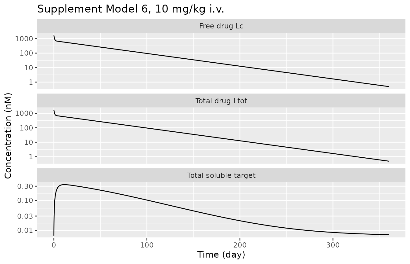
Removing the membrane target reduces Model 6 to the library’s QSS archetype
With the membrane target set to (numerically) zero, Model 6 is
exactly the two-compartment QSS TMDD model (Supplement Model 4). The
library already ships that structure as PK_2cmt_tmdd_qss,
written independently with a CL/V parameterisation and an amount-based
peripheral compartment. Mapping the Model 6 constants onto it
(CL = kel * Vc, Q = kpt * Vc,
Vp = Vc * kpt/ktp) must give the same total-drug profile.
This checks the central, peripheral and soluble-target equations of
Model 6 against a second, separately written implementation.
s6_nomem <- do.call(
  rxode2::rxSolve,
  c(list(m6, ev6, params = c(lrtot_mem = log(1e-15)), returnType = "data.frame"), tight)
)

kss <- (169 + 0.170) / 30.2 # Supplement Model 4/6: Kss = (koff + kep)/kon
arch <- readModelDb("PK_2cmt_tmdd_qss") |>
  rxode2::zeroRe() |>
  rxode2::ini(
    lcl = log(0.046 * VC), lvc = log(VC), lvp = log(VC * 0.902 / 0.725), lq = log(0.902 * VC),
    lT0 = log(0.00657), lkdeg = log(17.3), lkint = log(0.170), lkss = log(kss)
  )
s_arch <- do.call(rxode2::rxSolve, c(list(arch, ev6, returnType = "data.frame"), tight))

rel_arch <- max(abs(s_arch$Cc / s6_nomem$ctot - 1))
rel_arch
#> [1] 8.920642e-13
stopifnot(nrow(s_arch) == nrow(s6_nomem), rel_arch < 1e-6)
Drug mass balance
Drug leaves the body only through linear elimination of free drug, elimination of the soluble complex and the membrane-target Michaelis-Menten term, so the dose must equal the drug still in the body plus the cumulative eliminated flux. The flux is integrated with the trapezoidal rule on the dense log grid, which limits the closure to about 1e-5 (measured 6e-6).
flux6 <- with(s6, VC * (0.046 * Cc + total_target * 0.170 * Cc / (kss + Cc) +
  0.002 * 0.170 * Cc / ((169 + 0.170) / 30.2 + Cc)))
cum6 <- c(0, cumsum(diff(s6$time) * (head(flux6, -1) + tail(flux6, -1)) / 2))
closure6 <- (s6$central + s6$peripheral1 + cum6) / dose6 - 1
max(abs(closure6))
#> [1] 5.939772e-06
stopifnot(max(abs(closure6)) < 1e-4)
How much the membrane target contributes
The membrane term is a saturable extra elimination pathway, so
removing it can only raise exposure, and its share of elimination grows
as the dose falls and free drug approaches Kss_M (5.6 nM).
With the tutorial’s illustrative values the pathway is small at every
dose: the total membrane target is only Rm0 = 0.002 nM,
against free-drug concentrations of tens to thousands of nM.
auc_free <- function(sim) sum(diff(sim$time) * (head(sim$Cc, -1) + tail(sim$Cc, -1)) / 2)
dose_tab <- lapply(c(0.01, 0.1, 1, 10), function(d) {
  ev <- rxode2::et(amt = mgkg_to_nmolkg(d), cmt = "central") |> rxode2::et(grid6)
  with_m <- do.call(rxode2::rxSolve, c(list(m6, ev, returnType = "data.frame"), tight))
  no_m <- do.call(rxode2::rxSolve, c(list(m6, ev, params = c(lrtot_mem = log(1e-15)), returnType = "data.frame"), tight))
  tibble::tibble(
    `Dose (mg/kg)` = d,
    `Free-drug AUC with membrane target (nM day)` = auc_free(with_m),
    `Free-drug AUC without (nM day)` = auc_free(no_m)
  )
}) |>
  dplyr::bind_rows() |>
  dplyr::mutate(`Exposure lost to membrane target (%)` = 100 * (1 - `Free-drug AUC with membrane target (nM day)` / `Free-drug AUC without (nM day)`))
knitr::kable(dose_tab, digits = 3)| Dose (mg/kg) | Free-drug AUC with membrane target (nM day) | Free-drug AUC without (nM day) | Exposure lost to membrane target (%) |
|---|---|---|---|
| 0.01 | 36.008 | 36.052 | 0.122 |
| 0.10 | 360.232 | 360.530 | 0.083 |
| 1.00 | 3605.363 | 3606.300 | 0.026 |
| 10.00 | 36108.590 | 36110.250 | 0.005 |
lost <- dose_tab$`Exposure lost to membrane target (%)`
stopifnot(
  all(dose_tab$`Free-drug AUC with membrane target (nM day)` < dose_tab$`Free-drug AUC without (nM day)`),
  lost[1] > lost[4]
)
The membrane target removes 0.12% of free-drug exposure at 0.01 mg/kg
and 0.0046% at 10 mg/kg. Free-drug AUC is close to dose-proportional
across the whole range. With these values, neither target is abundant
enough to give the nonlinear profile TMDD is known for; raise
Rm0 or Rs0 to see it.
The supplement’s soluble-complex formula
The supplement computes the soluble complex as
Ps = Lctot - Lc - Rm0 * Lc / (Kssm + Lc), subtracting the
membrane-bound drug from total drug. But Lc comes from the
soluble-target quadratic, which solves
Lctot = Lc + Rstot * Lc / (Ksss + Lc) and so does not
include membrane-bound drug in Lctot. The two definitions
disagree by exactly the membrane-bound term,
Rm0 * Lc / (Kssm + Lc). The model file keeps the printed
form (complex_sol, target_sol) and adds the
QSS-consistent form (complex_sol_qss,
target_sol_qss). The identity below also confirms that the
quadratic is solved correctly at every time point.
bias <- with(s6, (complex_sol_qss - complex_sol) - 0.002 * Cc / ((169 + 0.170) / 30.2 + Cc))
max(abs(bias))
#> [1] 3.72387e-13
stopifnot(max(abs(bias)) < 1e-9)

s6 |>
  dplyr::select(time, `As printed (target_sol)` = target_sol, `QSS-consistent (target_sol_qss)` = target_sol_qss) |>
  tidyr::pivot_longer(-time) |>
  ggplot(aes(time, value, colour = name)) +
  geom_line() +
  labs(x = "Time (day)", y = "Free soluble target (nM)", colour = NULL) +
  theme(legend.position = "bottom")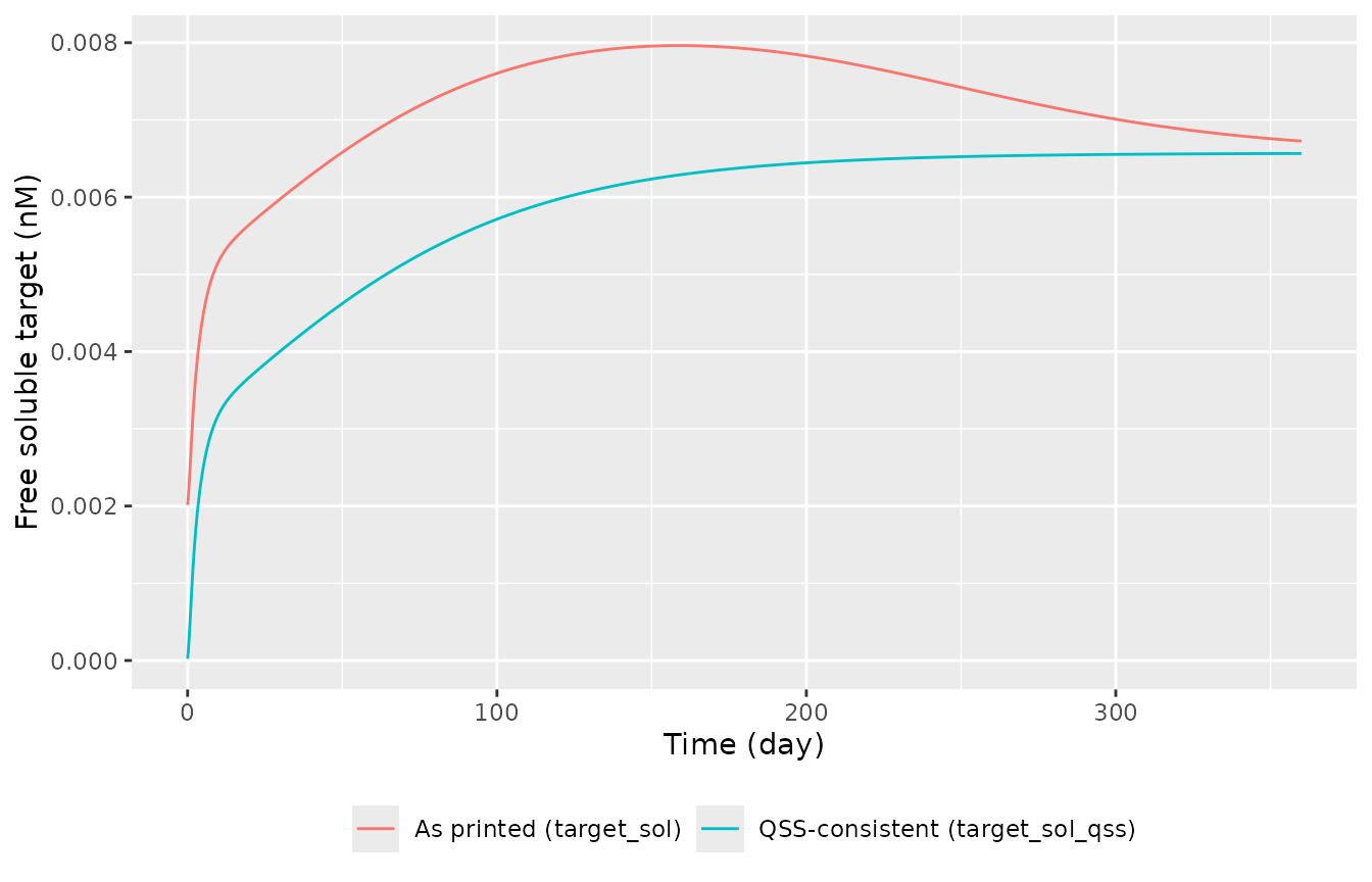
While drug is in excess the printed form understates the bound
soluble target by about Rm0 = 0.002 nM. The baseline is
only 0.00657 nM, so the printed free soluble target sits near 0.002 nM
where the QSS relation puts it close to zero. Use
target_sol_qss for target-suppression questions.
Model 7: full TMDD with FcRn recycling
Single dose, Lc0 = 200 nM (Supplement Model 7 regimen)
The supplement simulates 28 days.
grid7 <- sort(unique(c(0, seq(0, 28, by = 0.005))))
ev7 <- rxode2::et(amt = 200, cmt = "central") |> rxode2::et(grid7)
s7 <- do.call(rxode2::rxSolve, c(list(m7, ev7, returnType = "data.frame"), tight))

s7 |>
  dplyr::select(
    time,
    `Free drug, central` = central, `Free drug, tissue` = peripheral1,
    `Free target` = target, `Complex, central` = complex,
    `Endosomal drug, free` = endosome, `Endosomal drug, FcRn-bound` = endosome_fcrn,
    `Endosomal complex, free` = complex_endosome, `Endosomal complex, FcRn-bound` = complex_endosome_fcrn
  ) |>
  tidyr::pivot_longer(-time) |>
  ggplot(aes(time, value)) +
  geom_line() +
  facet_wrap(~name, scales = "free_y", ncol = 2) +
  labs(x = "Time (day)", y = "Concentration (nM)", title = "Supplement Model 7, Lc0 = 200 nM")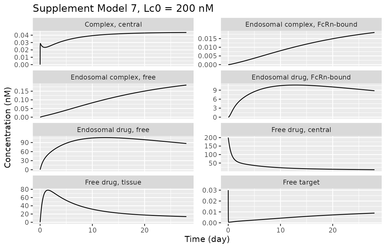
Drug mass balance
Summing the eight drug-containing equations, every binding, transfer,
uptake and recycling term cancels and only four elimination terms
remain: kelc * Lc + kepc * Pc + kele * Le + kele * Pe. So
the 200 nM dose must equal the drug left in the eight states plus the
integrated elimination.
drug7 <- with(s7, central + peripheral1 + complex + complex_peripheral1 +
  endosome + endosome_fcrn + complex_endosome + complex_endosome_fcrn)
flux7 <- with(s7, 0.024 * central + 0.201 * complex + 0.024 * endosome + 0.024 * complex_endosome)
cum7 <- c(0, cumsum(diff(s7$time) * (head(flux7, -1) + tail(flux7, -1)) / 2))
closure7 <- (drug7 + cum7) / 200 - 1
max(abs(closure7))
#> [1] 4.089254e-08
stopifnot(max(abs(closure7)) < 1e-6) # measured 4e-8
Switching off distribution and endosomal uptake reduces Model 7 to the one-compartment full TMDD archetype
With kup and kpt set to (numerically) zero,
no drug reaches the tissue or the endosome, and Model 7 is exactly the
one-compartment full TMDD model (Supplement Model 1, whose binding
constants Model 7 reuses). The library ships that structure as
PK_1cmt_tmdd_full. With Vc = 1 L and the dose
as 200 mg its central amount equals the Model 7 concentration, so the
two free-drug profiles must coincide.
s7_red <- do.call(
  rxode2::rxSolve,
  c(list(m7, ev7, params = c(lkup = log(1e-15), lk12 = log(1e-15)), returnType = "data.frame"), tight)
)
arch1 <- readModelDb("PK_1cmt_tmdd_full") |>
  rxode2::zeroRe() |>
  rxode2::ini(
    lcl = log(0.024), lvc = log(1), lT0 = log(0.03), lkdeg = log(0.823),
    lkint = log(0.201), lkon = log(0.592), lkoff = log(0.9)
  )
s_arch1 <- do.call(rxode2::rxSolve, c(list(arch1, ev7, returnType = "data.frame"), tight))

rel_arch1 <- max(abs(s_arch1$Cc / s7_red$Cc - 1))
rel_arch1
#> [1] 3.528289e-13
stopifnot(nrow(s_arch1) == nrow(s7_red), rel_arch1 < 1e-6)
What FcRn recycling does to exposure
Without FcRn, drug taken up into the endosome is lost: it is
eliminated there at kele and never returns. With FcRn, the
bound fraction is recycled to the central compartment, so central
exposure can only be higher.
s7_nofc <- do.call(
  rxode2::rxSolve,
  c(list(m7, ev7, params = c(lrtot_fcrn = log(1e-15)), returnType = "data.frame"), tight)
)
cmp7 <- dplyr::bind_rows(
  dplyr::mutate(s7, scenario = "FcRn 0.05 nM (Supplement Model 7)"),
  dplyr::mutate(s7_nofc, scenario = "No FcRn")
)
ggplot(cmp7, aes(time, Cc, colour = scenario)) +
  geom_line() +
  scale_y_log10() +
  labs(x = "Time (day)", y = "Free drug, central (nM)", colour = NULL) +
  theme(legend.position = "bottom")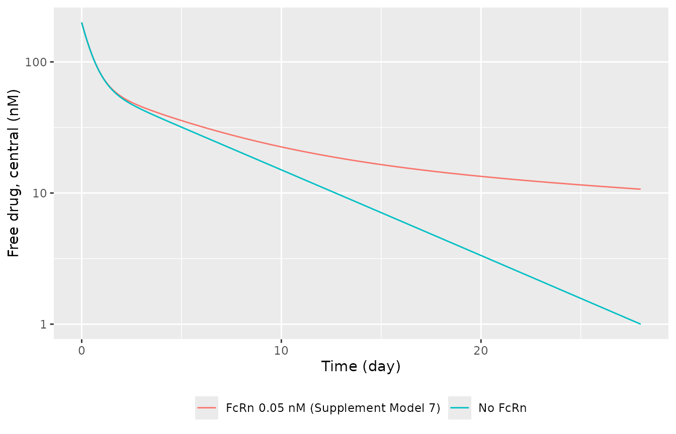
PKNCA on the free-drug profiles
The paper reports no NCA, so there is no published table to compare
against. PKNCA is run here on the deterministic free-drug profiles as a
descriptive summary, grouped by model and scenario. Model 7 is simulated
over the supplement’s 28-day horizon, so a large part of its
aucinf.obs is extrapolated.
conc_nca <- dplyr::bind_rows(
  dplyr::transmute(s6, id = 1L, treatment = "Model 6, 10 mg/kg", time, Cc),
  dplyr::transmute(s7, id = 2L, treatment = "Model 7, FcRn", time, Cc),
  dplyr::transmute(s7_nofc, id = 3L, treatment = "Model 7, no FcRn", time, Cc)
) |>
  dplyr::filter(!is.na(Cc))
dose_nca <- tibble::tibble(
  id = 1:3, time = 0,
  treatment = c("Model 6, 10 mg/kg", "Model 7, FcRn", "Model 7, no FcRn"),
  amt = c(dose6, 200, 200)
)
o_conc <- PKNCA::PKNCAconc(conc_nca, Cc ~ time | treatment + id)
o_dose <- PKNCA::PKNCAdose(dose_nca, amt ~ time | treatment + id, route = "intravascular")
intervals <- data.frame(start = 0, end = Inf, cmax = TRUE, aucinf.obs = TRUE, half.life = TRUE)
nca <- PKNCA::pk.nca(PKNCA::PKNCAdata(o_conc, o_dose, intervals = intervals))
summary(nca) |> knitr::kable()| start | end | treatment | N | cmax | half.life | aucinf.obs |
|---|---|---|---|---|---|---|
| 0 | Inf | Model 6, 10 mg/kg | 1 | 1670 | 34.1 | 36100 |
| 0 | Inf | Model 7, FcRn | 1 | 200 | 28.0 | 1150 |
| 0 | Inf | Model 7, no FcRn | 1 | 200 | 4.59 | 520 |
Assumptions and deviations
- Only two of the eight supplement models are in the library. Models 1-5 repeat structures the library already carries as TMDD archetypes, and Model 8 transcribes the Gibiansky 2012 denosumab estimates without that analysis’s variability and covariate model, so it is best taken from the primary paper.
- Illustrative parameters, not estimates. Neither model is fitted to data. Use them to explore model behaviour, not to predict any real antibody.
-
Model 6 is the i.v. form. Main-text Eqs V.1 and V.3
also carry a subcutaneous depot (
dLD/dt = -ka*LD,LD(0) = D1). Supplement Model 6 is i.v.-only and no absorption rate constant is printed anywhere, so no depot is included. (The input term of Eq V.3 is typesetkf LD; with the depot of Eq V.1 it is the absorption term.) -
Model 6 soluble-complex formula. The printed
Psis inconsistent with the quadratic that definesLc, by exactly the membrane-bound drug. Both forms are reported; see the section above. -
Model 7
kepeis unused. The supplement listskepe = 0.2011/day (“elimination of complex from endosome compartment”), but itsPeequation eliminates endosomal complex withkele = 0.0241/day, the same rate as endosomal free drug. The model file follows the equation. The main text describes the Xiao model as having equal elimination rates for drug and complex (ke(LC) = ke(PC)); the supplement applies that equality only in the endosome, while in the central compartment it keepskelc = 0.024andkepc = 0.2011/day.kepeis not carried inini()because no equation uses it. -
Model 7 FcRn is constant, and with these values that
assumption is stretched. Following Xiao 2010, the tutorial
holds FcRn fixed at
Fc0 = 0.05nM rather than tracking free FcRn. With the illustrative dose, the FcRn-bound drug pool reaches 10.7 nM, well above the stated FcRn concentration. A model that conserved FcRn would saturate the recycling pathway; this one does not. This is a property of the published model, reproduced as written. - Model 7 has no volume. Doses are concentrations (nM). To dose an amount, divide it by a central volume of your choosing; none is printed for Model 7.
-
No variability or residual error.
propSdisfixed(0)in both files. -
Integrator. The supplement integrates with
fourth-order Runge-Kutta at
DT = 0.01day. Here the models are solved with LSODA at tight tolerances.