Rifampicin multistate TB model in C57BL/6 mice (Chen 2017)
Source:vignettes/articles/Chen_2017_TB_MTP_rifampicin_mouse.Rmd
Chen_2017_TB_MTP_rifampicin_mouse.RmdModel and source
- Citation: Chen C, Ortega F, Rullas J, Alameda L, Angulo-Barturen I, Ferrer S, Simonsson USH. (2017). The multistate tuberculosis pharmacometric model: a semi-mechanistic pharmacokinetic-pharmacodynamic model for studying drug effects in an acute tuberculosis mouse model. J Pharmacokinet Pharmacodyn 44(2):133-141. doi:10.1007/s10928-017-9508-2. Final NONMEM control stream: Electronic Supplementary Material S2. Fixed rifampicin PK from Chen C, Ortega F, Alameda L, Ferrer S, Simonsson USH. Eur J Pharm Sci 93:319-333 (2016) doi:10.1016/j.ejps.2016.07.017; fixed MTP transfer rates from Clewe O, Aulin L, Hu Y, Coates AR, Simonsson USH. J Antimicrob Chemother 71(4):964-974 (2016) doi:10.1093/jac/dkv416.
- Description: Preclinical (C57BL/6 mouse). Multistate Tuberculosis Pharmacometric (MTP) model for rifampicin in an acute M. tuberculosis H37Rv lung-infection mouse model: a one-compartment first-order-absorption rifampicin PK model with auto-inducible clearance (fixed from a prior mouse popPK) drives an Emax inhibition of fast-multiplying bacterial growth, a sigmoid Emax stimulation of fast-multiplying bacterial death and a linear stimulation of slow-multiplying bacterial death in a three-state (fast-, slow-, non-multiplying) bacterial system; the CFU observation is the natural log of fast- plus slow-multiplying bacteria in the lungs.
- Article: https://doi.org/10.1007/s10928-017-9508-2
This is the single-drug rifampicin application of
the Multistate Tuberculosis Pharmacometric (MTP) model to an acute
M. tuberculosis H37Rv infection in C57BL/6 mice (Chen 2017,
J Pharmacokinet Pharmacodyn). It is a different paper from the
four-drug combination-therapy MTP-GPDI model in BALB/c mice (Chen 2017,
CPT:PSP; see Chen_2017_TB_MTP_GPDI_mouse).
Population
Sixty C57BL/6 mice were intratracheally infected with M. tuberculosis H37Rv (10^5 CFU per mouse) on Day 0. Twenty-five received oral rifampicin at 1.00, 2.83, 8.88, 26.4 or 98.0 mg/kg/day (five per dose) for eight days from Day 1 and were sacrificed on Day 9; twenty received 30 mg/kg/day for up to eight days and were sacrificed in groups of five on Days 2, 3, 4 and 9; fifteen untreated mice were sacrificed on Days 1, 9 and 18. The endpoint is colony-forming units (CFU) in the homogenised lungs, with a lower limit of quantification of 10 CFU/lungs (21.6% of observations were below it and were handled by the NONMEM M3 method).
No pharmacokinetics were sampled in this study. Rifampicin blood concentrations are predicted from an earlier mouse population-PK model with auto-induction (the population-PK-parameter approach), with every PK value held fixed. No interindividual variability was estimated.
rxode2::rxode2(readModelDb("Chen_2017_TB_MTP_rifampicin_mouse"))$population
#> $species
#> [1] "mouse (C57BL/6)"
#>
#> $n_subjects
#> [1] 60
#>
#> $n_studies
#> [1] 1
#>
#> $disease_state
#> [1] "Acute tuberculosis: intratracheal infection with M. tuberculosis H37Rv (10^5 CFU per mouse) on Day 0."
#>
#> $dose_range
#> [1] "Oral rifampicin once daily from Day 1 (24 h after infection): 1.00, 2.83, 8.88, 26.4 or 98.0 mg/kg/day for 8 days (5 mice per dose, sacrificed Day 9); 30 mg/kg/day for up to 8 days (5 mice sacrificed on each of Days 2, 3, 4 and 9); 15 untreated mice sacrificed on Days 1, 9 and 18 (5 per day)."
#>
#> $regions
#> [1] "GlaxoSmithKline Tres Cantos, Madrid, Spain"
#>
#> $notes
#> [1] "Chen 2017 Methods 'Rifampicin pharmacodynamic mouse study'. Endpoint is CFU in the homogenised lungs; LLOQ 10 CFU/lungs, 21.6% of observations below the LLOQ (handled by the NONMEM M3 method). No PK was sampled in this study: rifampicin blood concentrations come from the earlier mouse popPK model (population PK parameter approach) with every PK value fixed. No interindividual variability was estimated ($OMEGA 0 FIX in S2)."
Source trace
Every ini() entry carries an in-file comment pointing to
the Chen 2017 (or upstream) source location. The table below collects
them for reviewer use. The PK block is fixed from the upstream mouse
population-PK model; the MTP transfer rates kSF/kFN/kSN/kNS are fixed
from the in vitro Clewe 2016 fit; the growth, F0, kFSlin and the three
exposure-response relationships were estimated in this study.
| Block | Parameter | Value | Units | Source |
|---|---|---|---|---|
| RIF PK | lcl |
log(79.321) FIX | mL/h/kg | S2 $THETA(1); Methods 79.3 (Days 1-2) |
| RIF PK | lcl_late |
log(131.911) FIX | mL/h/kg | S2 $THETA(2); Methods 132 (Days >=3) |
| RIF PK | ltclchange |
log(48) FIX | h | S2 $PK IF(TIME.GE.48) |
| RIF PK | lvc |
log(1249.14) FIX | mL/kg | S2 $THETA(3); Methods 1250 (dose > 1.02 mg/kg) |
| RIF PK | lvc_lowdose |
log(2278.74) FIX | mL/kg | S2 $THETA(4); Methods 2280 (dose <= 1.02 mg/kg) |
| RIF PK | lka_excess |
log(0.994) FIX | 1/h | S2 $PK TVKA = KE + THETA(5) |
| RIF PK | lfdepot |
log(0.656) FIX | fraction | S2 $THETA(6); Methods 65.6% |
| MTP | lf0 |
log(331000) | CFU/lungs | Table 1 (treated mice), RSE 54.1% |
| MTP | lf0_untreated |
log(8340) | CFU/lungs | Table 1 (untreated mice), RSE 8.7% |
| MTP | lkg |
log(0.0333) | 1/h | Table 1, RSE 4.4% |
| MTP | lkfslin |
log(2.96e-5) | 1/h^2 | Table 1, RSE 29.8%; Eq. 1 |
| MTP | lksf |
log(6.042e-4) FIX | 1/h | Table 1 / S2 $THETA(12) (Clewe 2016, 0.0145/day /24) |
| MTP | lkfn |
log(3.7375e-8) FIX | 1/h | Table 1 / S2 $THETA(11) (Clewe 2016, 0.897e-6/day /24) |
| MTP | lksn |
log(7.75e-3) FIX | 1/h | Table 1 / S2 $THETA(13) (Clewe 2016, 0.186/day /24) |
| MTP | lkns |
log(5.125e-5) FIX | 1/h | Table 1 / S2 $THETA(14) (Clewe 2016, 0.123e-2/day /24) |
| RIF effect | lemax_fg_rif |
log(0.716) | fraction | Table 1 (FGImax), RSE 16.2%; Eq. 3 |
| RIF effect | lec50_fg_rif |
log(0.0397) | ug/mL | Table 1 (FGIC50), RSE 50.2% |
| RIF effect | gamma_fd_r |
2.19 | unitless | Table 1 (sigmoidicity), RSE 7.2% |
| RIF effect | lemax_fd_rif |
log(352) | 1/h | Table 1 (FDEmax), RSE 12.8%; Eq. 4 |
| RIF effect | lec50_fd_rif |
log(212) | ug/mL | Table 1 (FDEC50), RSE 30.4% |
| RIF effect | lksd_rif |
log(4.91e-3) | mL/(h*ug) | Table 1 (SDk), RSE 12.9%; Eq. 5 |
| Residual | propSd |
sqrt(0.0235) FIX | fraction | S2 first $SIGMA 0.0235 FIX (PK records; upstream popPK) |
| Residual | addSd |
sqrt(0.217) | log(CFU/lungs) | Table 1 (additive log-scale variance), RSE 12.0%; S2 second $SIGMA 0.216544 |
Equation references (recovered from the typeset equation GIFs and
confirmed against the S2 $DES block):
- Natural growth time-dependent transfer
kFS = kFSlin * t: Eq. 1. - Inhibition of fast-multiplying growth
IFG = FGImax * C / (FGIC50 + C): Eq. 3. - Stimulation of fast-multiplying death
EFD = FDEmax * C^gamma / (FDEC50^gamma + C^gamma): Eq. 4. - Stimulation of slow-multiplying death
ESD = SDk * C: Eq. 5. - Three-state ODE system for fast (F), slow (S), non-multiplying (N)
bacteria: Eqs. 6-8. The CFU observation is
log(F + S)(S2$ERROR:IPRED = LOG(A(3)+A(4))); non-multiplying N bacteria do not form colonies on solid media.
Virtual cohort and simulation
The model is deterministic and typical-value (no IIV, no dosing-level
random effects). Rifampicin is given once daily by oral gavage for eight
days from Day 1 (time = 24 h after infection,
addl = 7, ii = 24 h). The covariate
TRT_RIFAMPICIN selects the initial fast-multiplying
inoculum (331000 CFU/lungs treated vs 8340 untreated);
DOSE_LOW selects the larger apparent volume used for the
single 1 mg/kg cohort.
# The model has two endpoints (Cc and log_cfu) and no random effects. The
# typical-value solve uses sigma = NA rather than zeroRe(), which crashes on
# models with more than one endpoint.
mod <- readModelDb("Chen_2017_TB_MTP_rifampicin_mouse")

# One arm: observation rows on an ODE state (cmt = "central") with dvid = 1;
# rxode2 returns the bacterial states, Cc and log_cfu at those times.
# Rifampicin is dosed into the depot once daily for 8 days.
make_arm <- function(id, dose_mgkg, obs_days, treated = TRUE) {
  low <- as.numeric(dose_mgkg > 0 && dose_mgkg <= 1.02)
  obs <- data.frame(
    id = id, time = obs_days * 24, amt = 0, evid = 0L, cmt = "central",
    dvid = 1L, ii = 0, addl = 0L
  )
  dose <- NULL
  if (dose_mgkg > 0) {
    dose <- data.frame(
      id = id, time = 24, amt = dose_mgkg, evid = 1L, cmt = "depot",
      dvid = NA_integer_, ii = 24, addl = 7L
    )
  }
  ev <- rbind(obs, dose)
  ev$TRT_RIFAMPICIN <- as.numeric(treated)
  ev$DOSE_LOW <- low
  ev[order(ev$time, -ev$evid), ]
}

# Day-9 dose-response cohorts (Fig. 3) plus natural growth (Fig. 4a) and the
# 30 mg/kg longitudinal arm (Fig. 2, right).
day9_grid <- c(0, 1, 2, 4, 9)
events <- bind_rows(
  make_arm(0L, 0, c(0, 1, 9, 18), treated = FALSE),
  make_arm(1L, 1.00, day9_grid),
  make_arm(2L, 2.83, day9_grid),
  make_arm(3L, 8.88, day9_grid),
  make_arm(4L, 26.4, day9_grid),
  make_arm(5L, 98.0, day9_grid),
  make_arm(6L, 30.0, c(0, 2, 3, 4, 9))
)
dose_label <- c(
  "0" = "Natural growth", "1" = "1.00 mg/kg", "2" = "2.83 mg/kg",
  "3" = "8.88 mg/kg", "4" = "26.4 mg/kg", "5" = "98.0 mg/kg", "6" = "30 mg/kg"
)

sim <- rxode2::rxSolve(
  mod, events,
  keep = c("TRT_RIFAMPICIN", "DOSE_LOW"),
  returnType = "data.frame", sigma = NA, useLinCmt = FALSE,
  atol = 1e-14, rtol = 1e-12, maxsteps = 1e6
) |>
  as_tibble() |>
  mutate(
    day = time / 24,
    arm = dose_label[as.character(id)],
    log10_cfu = log10(pmax(fbugs + sbugs, 1))
  )
Replicate Figure S1 – typical rifampicin PK
Rifampicin blood concentration over 24 h after the Day-8 dose, across
the six dose levels. The peak concentrations and their roughly
dose-proportional spacing reproduce the supplement Figure S1
(1 -> ~0.3, 2.83 -> ~1.3,
8.88 -> ~4, 26.4 -> ~12,
30 -> ~13, 97.5 -> ~44 ug/mL).
pk_arm <- function(dose_mgkg) {
  low <- as.numeric(dose_mgkg <= 1.02)
  obs <- data.frame(
    id = 1L, time = 192 + seq(0, 24, by = 0.25), amt = 0, evid = 0L,
    cmt = "central", dvid = 1L
  )
  dose <- data.frame(
    id = 1L, time = seq(24, 192, by = 24), amt = dose_mgkg, evid = 1L,
    cmt = "depot", dvid = NA_integer_
  )
  ev <- rbind(obs, dose)
  ev$TRT_RIFAMPICIN <- 1
  ev$DOSE_LOW <- low
  s <- rxode2::rxSolve(
    mod, ev[order(ev$time, -ev$evid), ],
    returnType = "data.frame", sigma = NA, useLinCmt = FALSE,
    atol = 1e-12, rtol = 1e-10, maxsteps = 1e6
  )
  s <- s[s$time >= 192, ]
  tibble(tad = s$time - 192, Cc = s$Cc, dose = dose_mgkg)
}

pk <- bind_rows(lapply(c(1.00, 2.83, 8.88, 26.4, 30.0, 97.5), pk_arm)) |>
  mutate(dose = factor(dose))

ggplot(pk, aes(tad, Cc, colour = dose)) +
  geom_line(linewidth = 0.8) +
  scale_y_log10(name = "Predicted rifampicin blood concentration (ug/mL)") +
  scale_x_continuous(name = "Time after dose (hours)", breaks = seq(0, 24, 6)) +
  labs(
    title = "Replicates Figure S1 of Chen 2017",
    colour = "Dose (mg/kg)"
  ) +
  theme_minimal()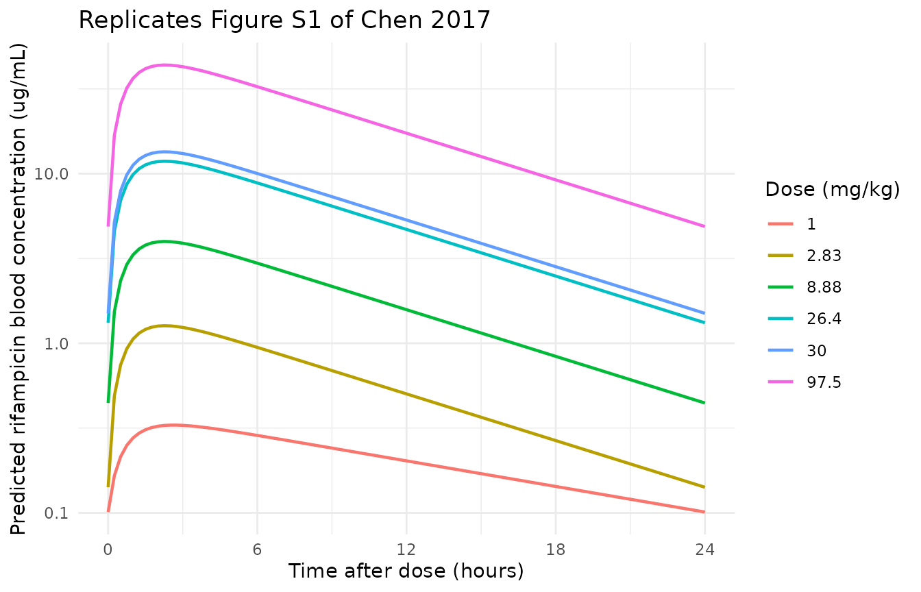
pk_peaks <- pk |>
  group_by(dose) |>
  summarise(Cmax = max(Cc), .groups = "drop")
pk_peaks |>
  dplyr::rename("Dose (mg/kg)" = dose, "Cmax (ug/mL)" = Cmax) |>
knitr::kable(digits = 2, caption = "Peak rifampicin blood concentration by dose (Day 8).")| Dose (mg/kg) | Cmax (ug/mL) |
|---|---|
| 1 | 0.33 |
| 2.83 | 1.27 |
| 8.88 | 3.98 |
| 26.4 | 11.84 |
| 30 | 13.46 |
| 97.5 | 43.74 |
Replicate Figure 4a – natural growth
With no drug, the fast-multiplying state grows exponentially and the slow- and non-multiplying populations follow from the transfer network. The total culturable CFU/lungs rises from the untreated inoculum (log10 ~ 3.9) to ~9 by Day 18, matching the Fig. 4a / Fig. 2 (left) observed medians of ~4.3, ~6.9 and ~9.1 at Days 1, 9 and 18.
ng <- sim |> filter(arm == "Natural growth")

ggplot(ng, aes(day, log10_cfu)) +
  geom_line(linewidth = 0.9) +
  geom_point(size = 2) +
  scale_y_continuous(name = "log10(CFU/lungs)", limits = c(3, 10)) +
  scale_x_continuous(name = "Time after infection (days)", breaks = c(1, 9, 18)) +
  labs(title = "Replicates Figure 4a of Chen 2017 (natural growth)") +
  theme_minimal()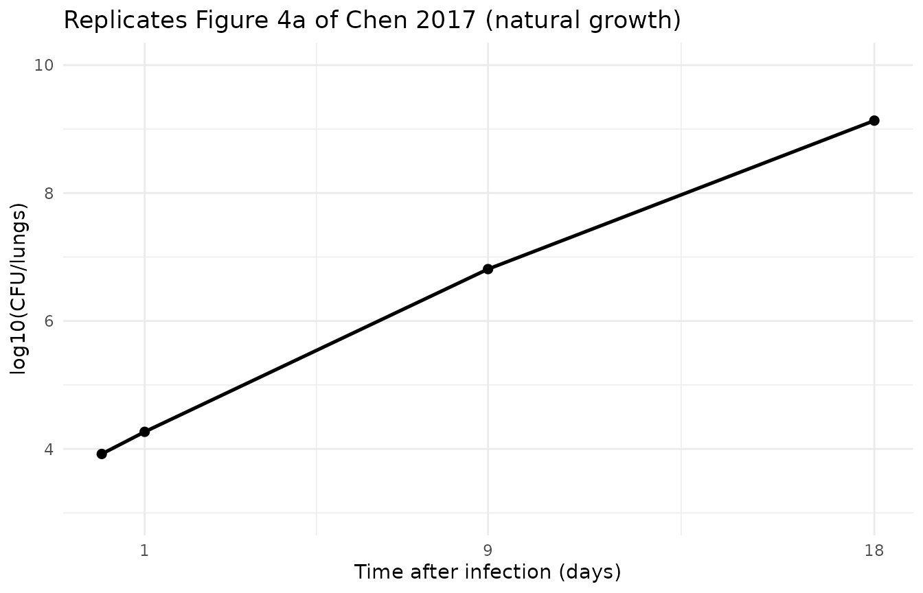
ng |>
  select(day, fbugs, sbugs, nbugs, log10_cfu) |>
  dplyr::rename(
    "Day" = day, "F" = fbugs, "S" = sbugs, "N" = nbugs,
    "log10(F+S)" = log10_cfu
  ) |>
  knitr::kable(
    digits = c(0, 0, 0, 0, 2),
    caption = "Natural-growth trajectory of the three bacterial states (CFU/lungs)."
)| Day | F | S | N | log10(F+S) |
|---|---|---|---|---|
| 0 | 8340 | 0 | 0 | 3.92 |
| 1 | 18389 | 116 | 6 | 4.27 |
| 9 | 5608537 | 867929 | 192928 | 6.81 |
| 18 | 973041879 | 383391107 | 116542906 | 9.13 |
Replicate Figure 3 – Day-9 dose-response
The predicted Day-9 culturable CFU/lungs falls monotonically with increasing rifampicin dose, reproducing the dose-response of Fig. 3 (observed medians ~6.8, ~5.2 and ~1.5 at 2.83, 8.88 and 26.4 mg/kg, with 30 and 97.5 mg/kg driven below the LLOQ).
d9 <- sim |>
  filter(id %in% 1:5, day == 9) |>
  mutate(dose_mgkg = c(1.00, 2.83, 8.88, 26.4, 98.0)[match(id, 1:5)])

ggplot(d9, aes(dose_mgkg, log10_cfu)) +
  geom_line(linewidth = 0.8) +
  geom_point(size = 2) +
  scale_x_log10(name = "Rifampicin dose (mg/kg/day)") +
  scale_y_continuous(name = "log10(CFU/lungs) at Day 9") +
  labs(title = "Replicates Figure 3 of Chen 2017 (Day 9 after infection)") +
  theme_minimal()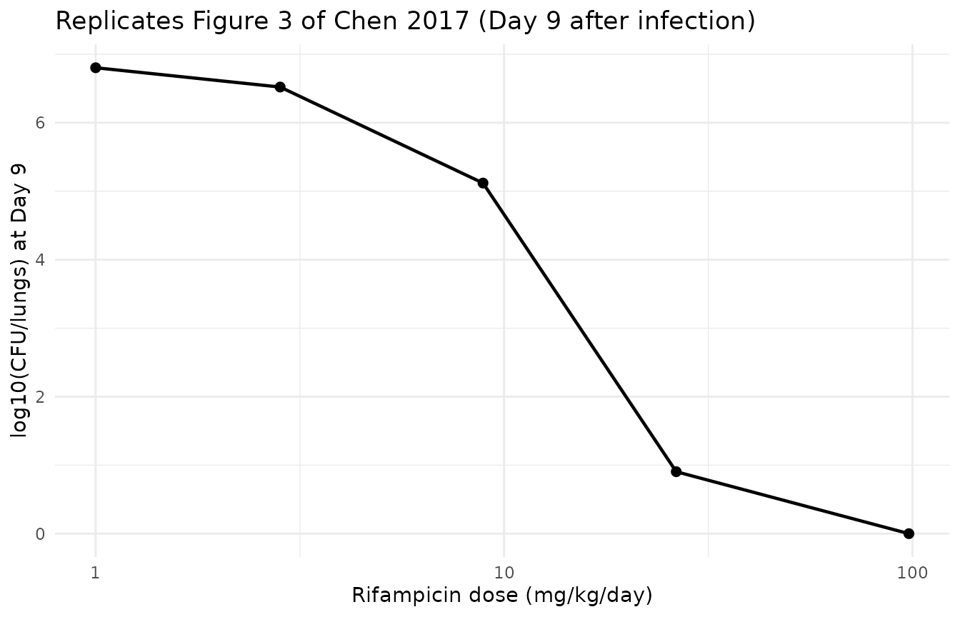
d9 |>
  select(dose_mgkg, log10_cfu) |>
  dplyr::rename("Dose (mg/kg)" = dose_mgkg, "log10(CFU/lungs) Day 9" = log10_cfu) |>
knitr::kable(digits = 2, caption = "Day-9 culturable CFU/lungs by rifampicin dose.")| Dose (mg/kg) | log10(CFU/lungs) Day 9 |
|---|---|
| 1.00 | 6.80 |
| 2.83 | 6.52 |
| 8.88 | 5.12 |
| 26.40 | 0.90 |
| 98.00 | 0.00 |
Replicate Figure 2 (right) – 30 mg/kg longitudinal decline
The 30 mg/kg arm, the only dose level with longitudinal sampling, declines from Day 2 to below the LLOQ by Day 9.
r30 <- sim |> filter(arm == "30 mg/kg", day > 0)

ggplot(r30, aes(day, log10_cfu)) +
  geom_line(linewidth = 0.9) +
  geom_point(size = 2) +
  geom_hline(yintercept = 1, linetype = "dashed", colour = "grey50") +
  scale_y_continuous(name = "log10(CFU/lungs)") +
  scale_x_continuous(name = "Time after infection (days)", breaks = c(2, 3, 4, 9)) +
  labs(
    title = "Replicates Figure 2 (right) of Chen 2017 (rifampicin 30 mg/kg)",
    caption = "Dashed line: LLOQ = 10 CFU/lungs (log10 = 1)."
  ) +
  theme_minimal()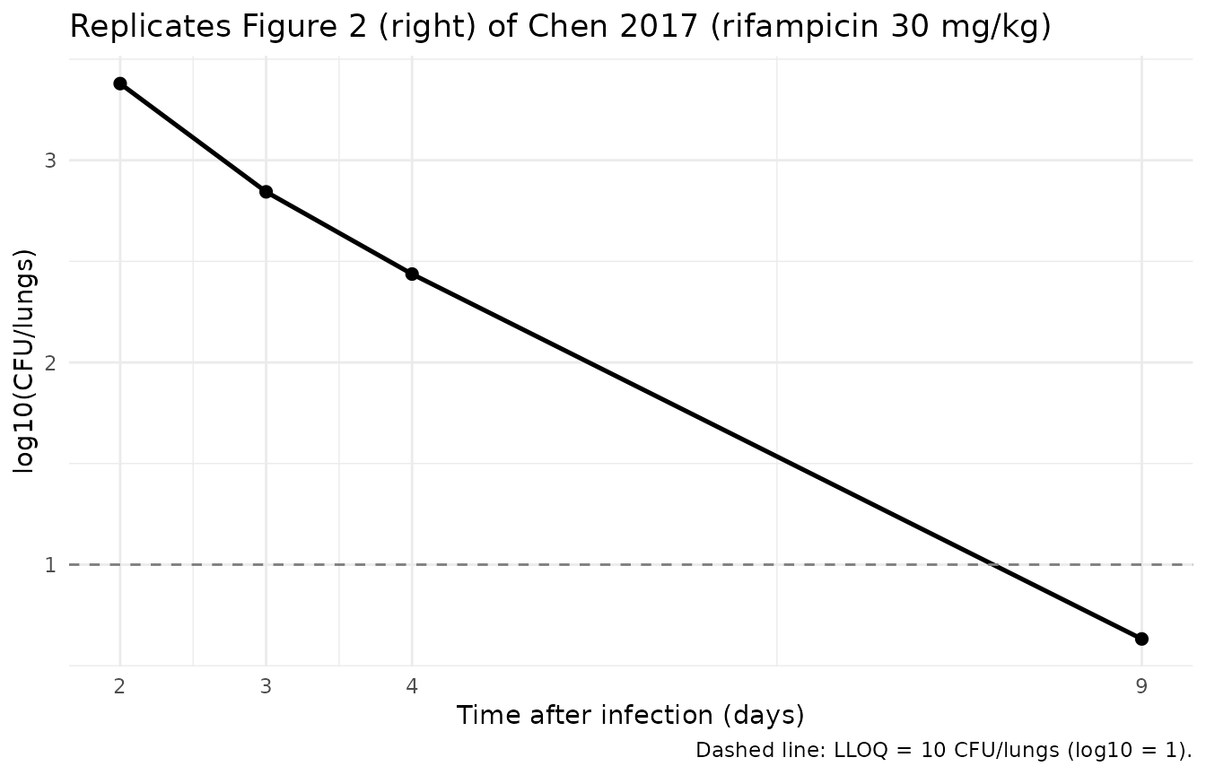
Validation checks
This is a deterministic, typical-value mechanistic model, so the checks below are exact (no stochastic cohort). They pin the structural behaviour against the published figures.
# 1. Natural growth rises monotonically to the observed Fig 4a medians.
ng_v <- ng |> arrange(day)
stopifnot(
  all(diff(ng_v$log10_cfu) > 0),
  abs(ng_v$log10_cfu[ng_v$day == 1] - 4.3) < 0.4,
  abs(ng_v$log10_cfu[ng_v$day == 9] - 6.9) < 0.4,
  abs(ng_v$log10_cfu[ng_v$day == 18] - 9.1) < 0.4
)

# 2. Day-9 dose-response is strictly decreasing across the five dose levels.
d9_v <- d9 |> arrange(dose_mgkg)
stopifnot(all(diff(d9_v$log10_cfu) < 0))

# 3. Day-9 predictions track the digitised Fig 3 medians for the quantifiable
#    cohorts (2.83 and 8.88 mg/kg).
stopifnot(
  abs(d9_v$log10_cfu[d9_v$dose_mgkg == 2.83] - 6.8) < 0.6,
  abs(d9_v$log10_cfu[d9_v$dose_mgkg == 8.88] - 5.2) < 0.6
)

# 4. 30 mg/kg declines over time and ends below the LLOQ by Day 9.
r30_v <- r30 |> arrange(day)
stopifnot(
  r30_v$log10_cfu[r30_v$day == 9] < r30_v$log10_cfu[r30_v$day == 2],
  r30_v$log10_cfu[r30_v$day == 9] < 1
)

# 5. Rifampicin Cmax rises monotonically with dose and the 1 mg/kg peak is sub-
#    ug/mL (Fig S1).
pk_v <- pk_peaks |> mutate(dose = as.numeric(as.character(dose))) |> arrange(dose)
stopifnot(
  all(diff(pk_v$Cmax) > 0),
  pk_v$Cmax[pk_v$dose == 1] < 1,
  abs(pk_v$Cmax[pk_v$dose == 97.5] - 44) < 8
)
Assumptions and deviations
-
Population-PK-parameter (PPP) approach. No
rifampicin PK was measured in this study. The entire PK block is fixed
from the upstream mouse population-PK model (Chen 2016, Eur J Pharm
Sci) and reproduced inline as
fixed()values; that upstream paper is not required because every value it contributes is carried here. -
Elimination-anchored absorption. The upstream PK
reparameterises absorption as
ka = kel + 0.994 /h(lka_excess), the standard NONMEM idiom enforcingka > kel. Becausekel = CL/Vis itself stratified by the auto-induction time step and by the lowest-dose volume,katakes several values, none of which is printed in the paper; the offset is therefore kept as a parameter rather than flattened to a singleka. -
Auto-induction clearance step. CL/F steps from 79.3
to 132 mL/h/kg at 48 h after infection
(
t >= exp(ltclchange)), per the S2IF(TIME.GE.48)branch. The model’s time axis is time since infection, matching the dataset (the fast-multiplying inoculum is set at time 0 and the first dose is at 24 h). The step therefore falls at the second dose. The Methods text and the Fig. 1 legend describe the lower clearance as applying on “Days 1-2”, and the$THETAcomments read “Days <= 2” / “Days >= 3”; those day labels number the dosing days of the upstream PK study, where a 48 h threshold falls at the third dose. The control stream is what produced the Table 1 estimates, so the 48 h step is encoded as written. -
Lowest-dose volume. The single 1.00 mg/kg cohort
(at or below the 1.02 mg/kg / 1020 ug/kg threshold) uses the larger
apparent volume 2278.74 mL/kg via
DOSE_LOW; all higher doses use 1249.14 mL/kg. -
Dose units. Doses are entered in mg/kg and the
apparent volume is in mL/kg, so
central / vcis in mg/mL; the model multiplies by 1000 to express the rifampicin blood concentrationCcin ug/mL (= mg/L), the units of the exposure-response EC50 values. -
CFU observation excludes the N state. The
culturable CFU is
log(F + S)(S2$ERROR), because non-multiplying bacteria do not form colonies on solid media. Thelog_cfuoutput is floored at 1 CFU to keep the log finite when drug effect drives the culturable total below one organism. -
No inoculum of slow- or non-multiplying bacteria.
The data did not support S0 or N0, so both are 0 at infection (Chen 2017
Results); only the fast-multiplying inoculum F0 is non-zero, and it
differs between treated
- and untreated (8340) mice.
- Fixed transfer rates. kSF, kFN, kSN and kNS are fixed to the in vitro Clewe 2016 estimates (per-day values divided by 24 to per-hour); only kFSlin was re-estimated as a time-dependent transfer in this mouse study.
- No rifampicin effect on the N state. An effect on non-multiplying bacteria was tested but not statistically significant (Chen 2017 Results), so none is encoded; the N state changes only through transfer.
-
Residual error scale. Table 1 reports the estimated
additive residual variance on the log scale as 0.217; with
log-transform-both-sides this is the natural-log CFU scale, so
addSd = sqrt(0.217). The control stream also carries a fixed proportional error on the rifampicin concentration ($SIGMA 0.0235 FIX, applied only to PK records, of which this study had none); it is kept aspropSd = sqrt(0.0235)onCcso the PK layer remains complete. - Near-zero initial amounts. The control stream initialises the depot, central, slow- and non-multiplying compartments at 1e-5 rather than 0 (a numerical convenience for the log of the CFU sum); the model starts them at 0, which changes the culturable count by far less than one CFU.
-
No interindividual variability.
$OMEGA 0 FIXin the control stream; the model is typical-value only. - 30 mg/kg Day-2 offset. The typical-value prediction at the first longitudinal time point (Day 2) sits below the observed median (~3.4 vs ~4.1 on the log10 scale); the decline shape to below the LLOQ by Day 9 and the Day-9 dose-response otherwise track the published figures.
Errata
- No erratum, corrigendum or author correction was identified for this
article via the EuropePMC
commentCorrectionList(null) or a PubMed “erratum” search as of 2026-10-15. - The final NONMEM control stream (Electronic Supplementary Material
S2) was used alongside Table 1: it is the only source that specifies the
PK block, the
ka = kel + offsetreparameterisation and theIPRED = log(F + S)observation. Two$THETAentries are initial estimates superseded by the published Table 1 finals (FDEmax 67.08 -> 352; FDEC50 98.50 -> 212); the Table 1 finals are used.