C-peptide kinetics and insulin secretion after IVGTT (Larizza 2018) • nlmixr2lib

library(nlmixr2lib)
library(rxode2)
library(dplyr)
library(ggplot2)

rxode2::rxSetSeed(20260923)

The paper

Larizza et al. (2018), CPT Pharmacometrics Syst Pharmacol 7(5):298-308, doi:10.1002/psp4.12285, presents a WinBUGS plugin for the DDMoRe Interoperability Framework. Its worked example is a complete, fully parameterised two-model pharmacometric workflow for assessing beta-cell function from an intravenous glucose tolerance test (IVGTT), and it is that workflow – not the software – that this article reproduces.

The workflow has three steps:

Fit a population regression that predicts the four macro constants of C-peptide two-compartment kinetics (short half-life ts, amplitude fraction F, long half-life tl, central volume V) from health status, sex, body surface area and age, in 207 subjects.
Simulate that regression for a new subject to obtain their individual C-peptide micro rate constants k01, k12, k21.
Fit the insulin minimal model to that new subject’s IVGTT C-peptide and glucose data, with the C-peptide kinetics taken from step 2, and read off the insulin secretion rate (ISR) and the beta-cell sensitivity indexes.

The paper runs this three times – a maximum-likelihood (MLE) route through NONMEM/PsN, a full-Bayesian route through WinBUGS, and a mixed route – which is why step 1 appears twice in the library, once per variability structure.

The three models

# modellib() returns the model function; rxode2() compiles it to the rxUi object
# whose `$theta`, `$state` and `$linCmt` slots the checks below inspect.
m0 <- rxode2::rxode2(modellib("Larizza_2018_cpeptideKinetics_M0"))
m4 <- rxode2::rxode2(modellib("Larizza_2018_cpeptideKinetics_M4"))
mm <- rxode2::rxode2(modellib("Larizza_2018_insulinMinimalModel"))

Model	Role in the workflow	Variability structure
`Larizza_2018_cpeptideKinetics_M0`	step 1, MLE route (approaches 1 and 3)	additive residual error on each macro constant; no IIV
`Larizza_2018_cpeptideKinetics_M4`	step 1, Bayesian route (approach 2)	full 4x4 interindividual covariance matrix; no residual error
`Larizza_2018_insulinMinimalModel`	step 3, all three approaches	proportional residual error, CV fixed at 6%

M0 and M4 are two versions of the same structural regression. With one observation of each macro constant per subject, a residual error and an interindividual covariance are not simultaneously identifiable, so the paper reports them in alternation – which is why Table 1’s sigma_ADD rows are blank in the M4 column and its xi rows are blank in the M0 column.

Population

The regression cohort is the 207-subject biosynthetic-C-peptide dataset of Van Cauter 1992 / Magni 2000, stratified as normal, obese or diabetic (type 2), with sex, age and body surface area recorded. Larizza 2018 does not reprint the per-stratum counts or the age and weight ranges.

The insulin minimal model is fitted to a single subject who is not in that cohort: normal health status, male, 25 years old, 1.818 m, 70.7 kg (Larizza 2018 Datasets section, citing Magni 2000 and Shapiro 1988). That subject’s basal plasma glucose is 87 mg/dL and their peak after the glucose bolus is 391 mg/dL; those two numbers are not in the main text but are carried explicitly in the deposited analysis scripts, and they are what the beta-cell sensitivity index phi1 is normalised by.

subject <- list(
  AGE = 25,
  SEXF = 0,
  DIS_OBESE = 0,
  DIS_DIAB = 0,
  height_m = 1.818,
  weight_kg = 70.7,
  glucose_basal_mgdl = 87,
  glucose_peak_mgdl = 391
)

# Larizza 2018 Mathematical Models: BSA = 0.20247 * Height(m)^0.725 * Weight(kg)^0.425
subject$BSA <-
  0.20247 * subject$height_m^0.725 * subject$weight_kg^0.425
subject$BSA
#> [1] 1.907961

Source trace

Every value in the three model files, and where it comes from.

Quantity	Model	Source
ts / F / tl / V regression equations	M0, M4	Mathematical Models, ‘A population regression model to estimate CP kinetic parameters’
BSA = 0.20247 * Ht^0.725 * Wt^0.425	M0, M4 (covariate note)	Mathematical Models, text below the regression equations
mtsn 5.000 / mtso 4.554 / mtsd 4.594 min	M0	Table 1, M0 column
mFn 0.764 / mFo 0.782 / mFd 0.780	M0	Table 1, M0 column
atl 27.797 min, btl 0.177 min/year	M0	Table 1, M0 column
aVm 0.495 L, bVm 1.982 L/m^2	M0	Table 1, M0 column
aVf 1.520 L, bVf 1.432 L/m^2	M0	Table 1, M0 column
sigma_ADD 1.143 / 0.041 / 5.778 / 0.846	M0	Table 1, M0 column; footnote c (‘SDs of the additive residual errors’)
mtsn 4.991 / mtso 4.496 / mtsd 4.693 min	M4	Table 1, M4 column
mFn 0.766 / mFo 0.781 / mFd 0.778	M4	Table 1, M4 column
atl 26.705 min, btl 0.209 min/year	M4	Table 1, M4 column
aVm 0.344 L, bVm 2.061 L/m^2	M4	Table 1, M4 column
aVf 0.795 L, bVf 1.819 L/m^2	M4	Table 1, M4 column
Xi, the 10 elements of the 4x4 covariance	M4	Table 1, M4 column; footnote b (‘Elements of the full matrix Xi’)
theta_0 / Sigma_0 / Wishart(q = 10, R) priors	M4 (model() comment)	Mathematical Models, Bayesian prior specification
k12 / k01 / k21 macro-to-micro equations	M0 (comment), MM	Mathematical Models, algebraic equations
k01 0.0607, k12 0.0491, k21 0.0503 /min	MM	Table 1, ‘CP-kinetic parameters’ (0.061 / 0.049 / 0.050); 4-digit values from Supporting Information 2, full-bayesian approach.R
CP1 / CP2 disposition ODEs	MM	Mathematical Models, ‘Glucose-insulin minimal model’, first subsystem
ISR = m*X; X, Y ODEs; X(0) = x0, Y(0) = 0	MM	Mathematical Models, second subsystem
m 0.817, alpha 0.061, beta 9.790 /min	MM	Table 2, MLE approach column
x0 1.384, h 89.002	MM	Table 2, MLE approach column
Residual CV fixed at 6%	MM	Mathematical Models, end of the minimal-model section
phi1 = (x0 * 10^3 / dG_mgdl) * 18.01; phi2 = beta	MM (comment), this article	Mathematical Models (definition); Supporting Information 2, MLE approach.R and full-bayesian approach.R (computational form)
Basal glucose 87 mg/dL, peak 391 mg/dL	this article	Supporting Information 2, full-bayesian approach.R: `phi1 <- ((coda_df$POP_x010^3)/(391-87))18.01`
Subject: normal, male, 25 y, 1.818 m, 70.7 kg	MM (population)	Datasets section

Step 1 and 2: the C-peptide kinetics regression

Closed-form check: the new subject’s macro and micro constants

This is the sharpest gate available on the whole workflow. The paper reports k01, k12 and k21 for the new subject in Table 1, and those values are the forward image of the M0 regression evaluated at that subject’s covariates followed by the macro-to-micro conversion. Nothing is fitted, nothing is sampled, and nothing depends on a dataset that is not available – so the reproduction must be exact to the printed precision.

cov_row <- data.frame(
  id = 1L,
  time = 0,
  cmt = c("thalfShort", "famp", "thalfLong", "vc"),
  evid = 0L,
  DIS_OBESE = subject$DIS_OBESE,
  DIS_DIAB = subject$DIS_DIAB,
  SEXF = subject$SEXF,
  BSA = subject$BSA,
  AGE = subject$AGE
)

m0_typ <- rxode2::rxSolve(rxode2::zeroRe(m0), cov_row, returnType = "data.frame")
#> Warning: No omega parameters in the model
macro <- m0_typ[1, c("thalfShort", "famp", "thalfLong", "vc")]
macro
#>   thalfShort  famp thalfLong       vc
#> 1          5 0.764    32.222 4.276579

# Larizza 2018 Mathematical Models: the macro-to-micro conversion. Kept out of
# model() (see the M0 file) because it is a post-processing step, and because a
# k12 / k21 / vc set inside an ODE-free model() risks rxode2 reading it as a
# solved linear system.
macro_to_micro <- function(ts, famp, tl) {
  k12 <- log(2) * (famp / tl + (1 - famp) / ts)
  k01 <- (log(2) / ts) * (log(2) / tl) * (1 / k12)
  k21 <- log(2) / ts + log(2) / tl - k12 - k01
  c(k01 = k01, k12 = k12, k21 = k21)
}

micro <- macro_to_micro(macro$thalfShort, macro$famp, macro$thalfLong)
micro
#>        k01        k12        k21 
#> 0.06067257 0.04915142 0.05031706

Reproduces the CP-kinetic-parameters block of Larizza 2018 Table 1.
Micro constant	Derived here (1/min)	Larizza 2018 Table 1 (1/min)	Supporting Information 2 (1/min)	Model ini() (1/min)
k01	0.06067	0.061	0.0607	0.0607
k12	0.04915	0.049	0.0491	0.0491
k21	0.05032	0.050	0.0503	0.0503

# The macro constants are exact functions of Table 1's printed fixed effects.
stopifnot(
  abs(macro$thalfShort - 5.000) < 1e-9,
  abs(macro$famp - 0.764) < 1e-9,
  abs(macro$thalfLong - 32.222) < 1e-9
)

# Against the paper's own 3-decimal Table 1 values.
stopifnot(all(abs(micro[c("k01", "k12", "k21")] - c(0.061, 0.049, 0.050)) < 5e-4))

The deposited scripts carry a digit more precision (0.0607 / 0.0491 / 0.0503), and that is what the minimal model fixes. Comparing against those needs a tolerance rather than an equality, because the fixed effects they were computed from are themselves printed rounded: NONMEM simulated M0 at its unrounded estimates, whereas the conversion above can only be fed Table 1’s three decimals. Rather than pick a tolerance by hand, propagate the printed rounding through the conversion and require the deposited values to lie inside the resulting interval.

half_ulp <- 5e-4 # Table 1 prints the fixed effects to three decimals

corners <- expand.grid(
  ts = 5.000 + c(-1, 1) * half_ulp,
  famp = 0.764 + c(-1, 1) * half_ulp,
  # tl = atl + btl * 25, so both rounding errors accumulate on the age slope
  tl = 32.222 + c(-1, 1) * (half_ulp + 25 * half_ulp)
)

envelope <- t(apply(corners, 1, function(r) {
  macro_to_micro(r[["ts"]], r[["famp"]], r[["tl"]])
}))

rng <- apply(envelope, 2, range)
rownames(rng) <- c("low", "high")
round(rng, 5)
#>          k01     k12     k21
#> low  0.06058 0.04908 0.05028
#> high 0.06076 0.04922 0.05035

deposited <- c(k01 = 0.0607, k12 = 0.0491, k21 = 0.0503)

stopifnot(
  all(deposited >= rng["low", names(deposited)]),
  all(deposited <= rng["high", names(deposited)]),
  # And the point conversion itself sits inside the same envelope.
  all(micro[names(deposited)] >= rng["low", names(deposited)]),
  all(micro[names(deposited)] <= rng["high", names(deposited)])
)

# Mutation control: a value one printed digit away must fall outside.
stopifnot(!(0.0481 >= rng["low", "k12"] && 0.0481 <= rng["high", "k12"]))

The three micro constants the minimal model fixes are therefore not free numbers: they follow from the M0 regression and the subject’s four covariates.

M0 is a regression, not a compartmental model

A guard worth stating explicitly, because both regression models define a parameter called vc and neither is a solved PK system:

stopifnot(
  is.null(m0$linCmt),
  is.null(m4$linCmt),
  length(m0$state) == 0L,
  length(m4$state) == 0L
)

M4: recovering the published covariance matrix

M4 places all of its stochastic structure in the 4x4 matrix Xi. Simulating a cohort and re-estimating the sample covariance of the four macro constants must return Xi, because the random effects enter additively on the natural scale.

n_sub <- 200L

cohort_cov <- data.frame(
  id = seq_len(n_sub),
  DIS_OBESE = 0,
  DIS_DIAB = 0,
  SEXF = 0,
  BSA = subject$BSA,
  AGE = subject$AGE
)

cohort_ev <- merge(
  cohort_cov,
  data.frame(
    time = 0,
    cmt = c("thalfShort", "famp", "thalfLong", "vc"),
    evid = 0L
  )
)

m4_sim <- rxode2::rxSolve(m4, cohort_ev, returnType = "data.frame")

macro_draws <- m4_sim |>
  dplyr::filter(!duplicated(id)) |>
  dplyr::select(thalfShort, famp, thalfLong, vc)

xi_published <- matrix(
  c(
    1.295, 0.006, 3.250, 0.596,
    0.006, 0.002, 0.071, -0.006,
    3.250, 0.071, 33.044, 1.915,
    0.596, -0.006, 1.915, 0.713
  ),
  nrow = 4, byrow = TRUE,
  dimnames = list(
    c("ts", "F", "tl", "V"),
    c("ts", "F", "tl", "V")
  )
)

xi_sim <- stats::cov(as.matrix(macro_draws))
dimnames(xi_sim) <- dimnames(xi_published)
round(xi_sim, 4)
#>        ts       F      tl       V
#> ts 1.4550  0.0046  3.0523  0.6650
#> F  0.0046  0.0021  0.0423 -0.0083
#> tl 3.0523  0.0423 34.4227  1.9137
#> V  0.6650 -0.0083  1.9137  0.7540

# The published matrix must be a valid covariance in the first place.
stopifnot(!inherits(try(chol(xi_published), silent = TRUE), "try-error"))

# Compare on the correlation scale plus the variance ratios, so one comparison
# is not dominated by the 16,000-fold spread in the variances themselves. With
# 200 draws the Monte-Carlo standard error on a correlation is about 0.07, so
# the tolerances below are loose by construction; they catch a transposed or
# mis-ordered Xi, not small sampling noise.
cor_pub <- stats::cov2cor(xi_published)
cor_sim <- stats::cov2cor(xi_sim)
off <- upper.tri(cor_pub)

var_ratio <- diag(xi_sim) / diag(xi_published)

stopifnot(
  max(abs(cor_sim[off] - cor_pub[off])) < 0.25,
  all(var_ratio > 0.6), all(var_ratio < 1.6)
)

# The typical values must be untouched by the random effects.
stopifnot(
  abs(mean(macro_draws$thalfShort) - 4.991) < 0.25,
  abs(mean(macro_draws$famp) - 0.766) < 0.01
)

Correlations implied by Xi (Larizza 2018 Table 1, M4 column) against a 200-subject simulation.
Pair	Published correlation	Simulated correlation
ts-F	0.118	0.083
ts-tl	0.497	0.431
ts-V	0.276	0.158
F-tl	0.620	0.635
F-V	-0.159	-0.209
tl-V	0.395	0.376

What the regression says across the covariate space

Replicates the covariate relationships behind Larizza 2018 Supplementary Figures S2 and S5 (VPCs of the four macro constants against hstatus, AGE and BSA).

grid <- expand.grid(
  AGE = seq(20, 80, by = 5),
  status = c("normal", "obese", "diabetic"),
  SEXF = c(0, 1),
  stringsAsFactors = FALSE
) |>
  dplyr::mutate(
    DIS_OBESE = as.numeric(status == "obese"),
    DIS_DIAB = as.numeric(status == "diabetic"),
    BSA = subject$BSA,
    id = dplyr::row_number()
  )

grid_ev <- merge(
  grid,
  data.frame(time = 0, cmt = c("thalfShort", "famp", "thalfLong", "vc"), evid = 0L)
)

grid_out <- rxode2::rxSolve(rxode2::zeroRe(m0), grid_ev, returnType = "data.frame") |>
  dplyr::filter(!duplicated(id)) |>
  # Join only `status`; AGE and SEXF come back from the solve itself, so joining
  # them again would produce .x / .y suffixes instead of the columns used below.
  dplyr::left_join(dplyr::select(grid, id, status), by = "id") |>
  dplyr::rowwise() |>
  dplyr::mutate(
    k01 = macro_to_micro(thalfShort, famp, thalfLong)[["k01"]]
  ) |>
  dplyr::ungroup()
#> Warning: No omega parameters in the model
#> Warning: multi-subject simulation without without 'omega'

stopifnot(all(c("AGE", "SEXF", "status", "k01") %in% names(grid_out)))

ggplot(
  grid_out,
  aes(AGE, k01, colour = status, linetype = factor(SEXF, labels = c("male", "female")))
) +
  geom_line(linewidth = 0.8) +
  labs(
    x = "Age (years)",
    y = expression(k[" 01"] ~ "(1/min)"),
    colour = "Health status",
    linetype = "Sex",
    title = "M0-predicted C-peptide elimination rate constant"
  ) +
  theme_bw()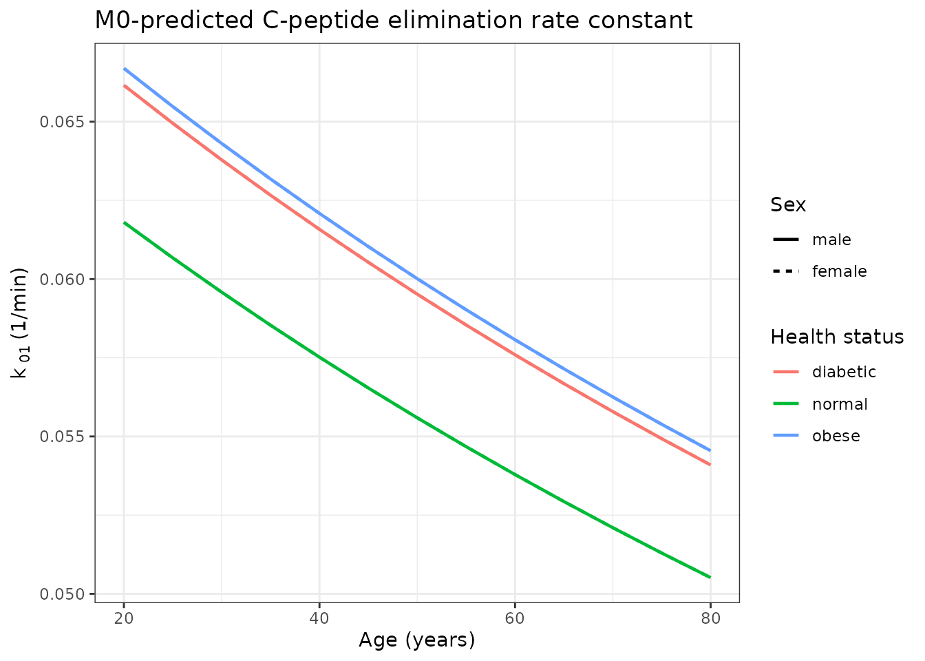

k01 does not depend on sex, because sex enters only the volume regression and the macro-to-micro conversion does not use the volume – a small structural check that the conversion has been wired up correctly.

Step 3: the insulin minimal model

The glucose forcing function

The minimal model takes plasma glucose as an error-free time-varying regressor; it does not model glucose kinetics. The subject’s actual glucose series was not available, so the profile below is illustrative. It is anchored on the two glucose values that are recoverable from the sources (basal 87 mg/dL, peak 391 mg/dL) and given a conventional bi-exponential IVGTT return to basal. Every numeric assertion in this article is chosen to be independent of this choice – see “Assumptions and deviations”.

The time grid is the one the deposited scripts use for ISR simulation: c(seq(0, 10, 0.05), seq(10, 240, 5)), refined here in the tail so the figures are smooth.

tgrid <- sort(unique(c(seq(0, 10, by = 0.05), seq(10, 240, by = 1))))

ivgtt_glucose <- function(t, basal = 87, peak = 391, tpeak = 2,
                          frac_fast = 0.55, k_fast = 0.12, k_slow = 0.022) {
  delta <- peak - basal
  ifelse(
    t < tpeak,
    basal + delta * t / tpeak,
    basal + delta * (frac_fast * exp(-k_fast * (t - tpeak)) +
      (1 - frac_fast) * exp(-k_slow * (t - tpeak)))
  )
}

glucose <- data.frame(time = tgrid, GLU = ivgtt_glucose(tgrid))

ggplot(glucose, aes(time, GLU)) +
  geom_line(linewidth = 0.8) +
  geom_hline(yintercept = 89.002, linetype = "dashed", colour = "grey40") +
  annotate("text", x = 180, y = 100, label = "h = 89.0 mg/dL (MLE)", size = 3, colour = "grey30") +
  labs(
    x = "Time (min)", y = "Plasma glucose (mg/dL)",
    title = "Illustrative IVGTT glucose forcing function",
    subtitle = "Anchored on the paper's basal 87 and peak 391 mg/dL"
  ) +
  theme_bw()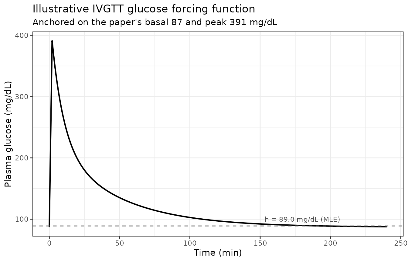

The three approaches

Larizza 2018 Table 2 reports the minimal model under all three approaches. The library model carries the MLE column; the other two are one ini() call away.

approaches <- list(
  MLE = c(msecr = 0.817, alpha = 0.061, beta = 9.790, x0 = 1.384, gthresh = 89.002),
  Bayesian = c(msecr = 0.820, alpha = 0.051, beta = 10.498, x0 = 1.472, gthresh = 89.097),
  Mixed = c(msecr = 0.907, alpha = 0.074, beta = 8.909, x0 = 1.406, gthresh = 89.859)
)

mm_variant <- function(p) {
  rxode2::ini(
    mm,
    msecr = unname(p[["msecr"]]),
    alpha = unname(p[["alpha"]]),
    beta = unname(p[["beta"]]),
    x0 = unname(p[["x0"]]),
    gthresh = unname(p[["gthresh"]])
  )
}

# Confirm ini() actually took: element assignment into a model's theta is a
# silent no-op in rxode2, so the piped result is checked rather than assumed.
mm_mixed <- mm_variant(approaches$Mixed)
#> ℹ change initial estimate of `msecr` to `0.907`
#> ℹ change initial estimate of `alpha` to `0.074`
#> ℹ change initial estimate of `beta` to `8.909`
#> ℹ change initial estimate of `x0` to `1.406`
#> ℹ change initial estimate of `gthresh` to `89.859`
stopifnot(
  abs(unname(mm_mixed$theta[["msecr"]]) - 0.907) < 1e-12,
  abs(unname(mm_mixed$theta[["gthresh"]]) - 89.859) < 1e-12,
  abs(unname(mm$theta[["msecr"]]) - 0.817) < 1e-12
)

solve_mm <- function(p, glu = glucose) {
  ev <- data.frame(
    id = 1L,
    time = glu$time,
    evid = 0L,
    cmt = "central",
    GLU = glu$GLU
  )
  rxode2::rxSolve(rxode2::zeroRe(mm_variant(p)), ev, returnType = "data.frame")
}

sims <- lapply(names(approaches), function(nm) {
  out <- solve_mm(approaches[[nm]])
  out$approach <- nm
  out
})
#> ℹ change initial estimate of `msecr` to `0.817`
#> ℹ change initial estimate of `alpha` to `0.061`
#> ℹ change initial estimate of `beta` to `9.79`
#> ℹ change initial estimate of `x0` to `1.384`
#> ℹ change initial estimate of `gthresh` to `89.002`
#> Warning: No omega parameters in the model
#> ℹ change initial estimate of `msecr` to `0.82`
#> ℹ change initial estimate of `alpha` to `0.051`
#> ℹ change initial estimate of `beta` to `10.498`
#> ℹ change initial estimate of `x0` to `1.472`
#> ℹ change initial estimate of `gthresh` to `89.097`
#> Warning: No omega parameters in the model
#> ℹ change initial estimate of `msecr` to `0.907`
#> ℹ change initial estimate of `alpha` to `0.074`
#> ℹ change initial estimate of `beta` to `8.909`
#> ℹ change initial estimate of `x0` to `1.406`
#> ℹ change initial estimate of `gthresh` to `89.859`
#> Warning: No omega parameters in the model
sims <- dplyr::bind_rows(sims)
sims$approach <- factor(sims$approach, levels = names(approaches))

stopifnot(!anyNA(sims$Cc), !anyNA(sims$ISR), all(sims$ISR >= 0))

Replicating Figure 4

Larizza 2018 Figure 4 panels a-c show the C-peptide fit under each approach and panels d-f show the reconstructed ISR over [0, 1], [1, 5] and [5, 240] minutes. The three time windows exist because the first-phase burst and the second-phase provision act on very different timescales.

ggplot(sims, aes(time, Cc, colour = approach)) +
  geom_line(linewidth = 0.8) +
  labs(
    x = "Time (min)",
    y = "C-peptide above basal (model units)",
    colour = "Approach",
    title = "Replicates Figure 4a-c of Larizza 2018",
    subtitle = "Baseline-subtracted plasma C-peptide under the three approaches"
  ) +
  theme_bw()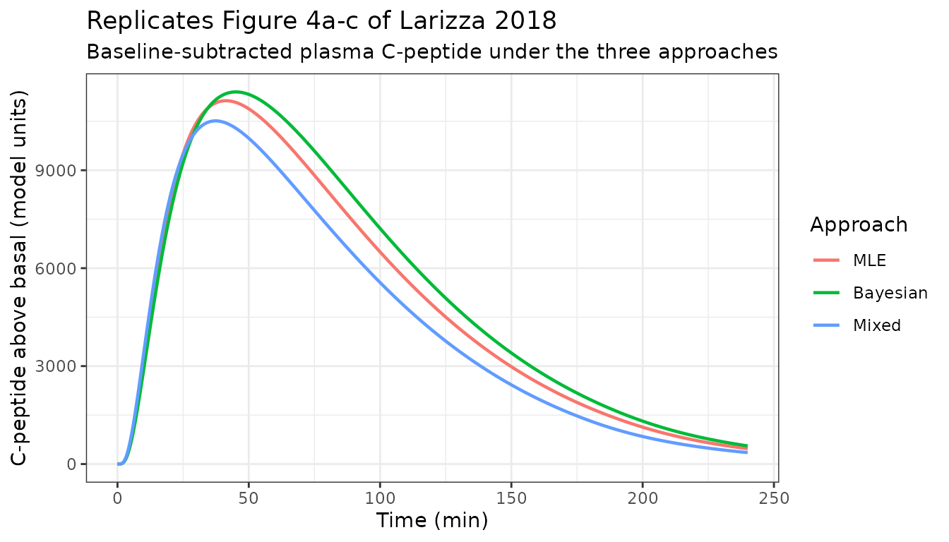

windows <- list(
  "d: 0-1 min" = c(0, 1),
  "e: 1-5 min" = c(1, 5),
  "f: 5-240 min" = c(5, 240)
)

isr_panels <- dplyr::bind_rows(lapply(names(windows), function(w) {
  lo <- windows[[w]][1]
  hi <- windows[[w]][2]
  sims |>
    dplyr::filter(time >= lo, time <= hi) |>
    dplyr::mutate(panel = w)
}))
isr_panels$panel <- factor(isr_panels$panel, levels = names(windows))

ggplot(isr_panels, aes(time, ISR, colour = approach)) +
  geom_line(linewidth = 0.8) +
  facet_wrap(~panel, scales = "free") +
  labs(
    x = "Time (min)", y = "ISR (model units / min)", colour = "Approach",
    title = "Replicates Figure 4d-f of Larizza 2018",
    subtitle = "Insulin secretion rate over the paper's three time windows"
  ) +
  theme_bw() +
  theme(legend.position = "bottom")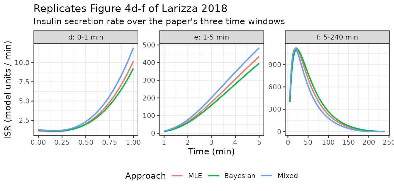

Validation

The minimal model’s subject-level dataset was not available, so none of the checks below leans on a simulated magnitude. Each is either a closed-form identity, a conservation law, or arithmetic on the paper’s own printed numbers.

1. First-phase closed form

Below the glucose threshold the provision factor is never stimulated, so Y(t) = 0 for all time and the secretion subsystem collapses to a single exponential: X(t) = x0 * exp(-m * t) and ISR(t) = m * x0 * exp(-m * t). The total first-phase secretion is then exactly x0, whatever m is.

flat <- data.frame(time = tgrid, GLU = 80) # strictly below every approach's h

first_phase <- solve_mm(approaches$MLE, flat)
#> ℹ change initial estimate of `msecr` to `0.817`
#> ℹ change initial estimate of `alpha` to `0.061`
#> ℹ change initial estimate of `beta` to `9.79`
#> ℹ change initial estimate of `x0` to `1.384`
#> ℹ change initial estimate of `gthresh` to `89.002`
#> Warning: No omega parameters in the model

analytic_x <- approaches$MLE[["x0"]] * exp(-approaches$MLE[["msecr"]] * first_phase$time)

stopifnot(
  # Provision is identically zero, never merely small.
  max(abs(first_phase$provision)) < 1e-10,
  # The beta-cell store follows the analytic exponential.
  max(abs(first_phase$betacell - analytic_x)) < 1e-6,
  # ISR = m * X exactly.
  max(abs(first_phase$ISR - approaches$MLE[["msecr"]] * first_phase$betacell)) < 1e-9
)

# Cumulative first-phase secretion -> x0 as t -> Inf.
released <- approaches$MLE[["x0"]] - utils::tail(first_phase$betacell, 1)
c(released = released, x0 = approaches$MLE[["x0"]])
#> released       x0 
#>    1.384    1.384
stopifnot(abs(released - approaches$MLE[["x0"]]) < 1e-9)

A mutation control, so the check above is demonstrably not vacuous: raising the glucose input above the threshold must break the closed form.

stimulated <- solve_mm(approaches$MLE, data.frame(time = tgrid, GLU = 120))
#> ℹ change initial estimate of `msecr` to `0.817`
#> ℹ change initial estimate of `alpha` to `0.061`
#> ℹ change initial estimate of `beta` to `9.79`
#> ℹ change initial estimate of `x0` to `1.384`
#> ℹ change initial estimate of `gthresh` to `89.002`
#> Warning: No omega parameters in the model
stopifnot(max(abs(stimulated$provision)) > 1)

2. C-peptide mass balance

Everything the beta cells secrete must end up either eliminated through k01 or still present in the two C-peptide compartments. Integrating the flux terms as extra ODE states makes the identity exact to solver tolerance rather than to trapezoidal-rule error – which matters here, because ISR has a sharp spike in the first minute that a coarse trapezoid would badly mis-integrate.

mm_auc <- mm |>
  rxode2::model({
    d/dt(auc_isr) <- ISR
    d/dt(auc_cp1) <- central
  }, append = TRUE)

ev_mb <- data.frame(
  id = 1L, time = glucose$time, evid = 0L, cmt = "central", GLU = glucose$GLU
)
mb <- rxode2::rxSolve(rxode2::zeroRe(mm_auc), ev_mb, returnType = "data.frame")
#> Warning: No omega parameters in the model

k01_mm <- exp(unname(mm$theta[["lk01"]]))

secreted <- mb$auc_isr
eliminated <- k01_mm * mb$auc_cp1
retained <- mb$central + mb$peripheral1
residual <- secreted - (eliminated + retained)

# Absolute closure, and closure relative to the amount that has moved.
c(
  max_abs_residual = max(abs(residual)),
  max_rel_residual = max(abs(residual[-1]) / secreted[-1])
)
#> max_abs_residual max_rel_residual 
#>     2.619345e-10     3.601195e-15

# Observed closure is around 1e-15 relative, so the bound below leaves seven
# orders of margin while still being far tighter than trapezoidal integration
# of the first-minute ISR spike could ever achieve.
stopifnot(max(abs(residual[-1]) / secreted[-1]) < 1e-8)

The same mutation control: a deliberately wrong elimination constant must break the balance.

bad <- secreted - (2 * k01_mm * mb$auc_cp1 + retained)
stopifnot(max(abs(bad[-1]) / secreted[-1]) > 0.1)

3. The threshold switch

h is an estimated parameter, so the model must be genuinely inert at and below it and responsive above it.

at_threshold <- solve_mm(
  approaches$MLE,
  data.frame(time = tgrid, GLU = approaches$MLE[["gthresh"]])
)
#> ℹ change initial estimate of `msecr` to `0.817`
#> ℹ change initial estimate of `alpha` to `0.061`
#> ℹ change initial estimate of `beta` to `9.79`
#> ℹ change initial estimate of `x0` to `1.384`
#> ℹ change initial estimate of `gthresh` to `89.002`
#> Warning: No omega parameters in the model
just_above <- solve_mm(
  approaches$MLE,
  data.frame(time = tgrid, GLU = approaches$MLE[["gthresh"]] + 10)
)
#> ℹ change initial estimate of `msecr` to `0.817`
#> ℹ change initial estimate of `alpha` to `0.061`
#> ℹ change initial estimate of `beta` to `9.79`
#> ℹ change initial estimate of `x0` to `1.384`
#> ℹ change initial estimate of `gthresh` to `89.002`
#> Warning: No omega parameters in the model

stopifnot(
  max(abs(at_threshold$provision)) < 1e-10,
  # Steady-state provision above threshold is beta * (G - h), reached to machine
  # precision after 240 min, which is ~15 time constants (1/alpha = 16.4 min).
  abs(utils::tail(just_above$provision, 1) - approaches$MLE[["beta"]] * 10) /
    (approaches$MLE[["beta"]] * 10) < 1e-6
)

4. Beta-cell sensitivity indexes

phi1 and phi2 are the paper’s headline read-outs. phi2 is just beta, so it must reproduce exactly. phi1 is x0 divided by the maximum glucose increment; the main text gives the definition and the deposited scripts give the computational form, including the 18.01 g/mol conversion from mg/dL to mmol/L and the 10^3 scaling.

delta_g_mgdl <- subject$glucose_peak_mgdl - subject$glucose_basal_mgdl
delta_g_mgdl
#> [1] 304

phi1_of <- function(x0) (x0 * 1e3 / delta_g_mgdl) * 18.01

index_table <- tibble::tibble(
  Approach = names(approaches),
  x0 = vapply(approaches, function(p) unname(p[["x0"]]), numeric(1)),
  beta = vapply(approaches, function(p) unname(p[["beta"]]), numeric(1))
) |>
  dplyr::mutate(
    `phi1 (derived)` = round(phi1_of(x0), 3),
    `phi1 (Table 2)` = c(81.966, 87.177, 83.314),
    `phi2 (derived)` = beta,
    `phi2 (Table 2)` = c(9.790, 10.498, 8.909)
  ) |>
  dplyr::select(Approach, x0, `phi1 (derived)`, `phi1 (Table 2)`, `phi2 (derived)`, `phi2 (Table 2)`)

knitr::kable(index_table, caption = "Reproduces the u1 and u2 rows of Larizza 2018 Table 2.")

Reproduces the u1 and u2 rows of Larizza 2018 Table 2.
Approach	x0	phi1 (derived)	phi1 (Table 2)	phi2 (derived)	phi2 (Table 2)
MLE	1.384	81.993	81.966	9.790	9.790
Bayesian	1.472	87.206	87.177	10.498	10.498
Mixed	1.406	83.296	83.314	8.909	8.909

stopifnot(
  # phi2 = beta is an identity and must be exact.
  all(index_table$`phi2 (derived)` == index_table$`phi2 (Table 2)`),
  # phi1 is reconstructed from x0 rounded to 3 decimals in Table 2, so the
  # residual is pure print-rounding: 0.001 pmol/L of x0 moves phi1 by 0.06.
  max(abs(index_table$`phi1 (derived)` - index_table$`phi1 (Table 2)`)) < 0.1
)

# phi2 is also emitted by the model itself.
stopifnot(
  all(abs(
    tapply(sims$phi2, sims$approach, function(x) x[1]) -
      c(9.790, 10.498, 8.909)
  ) < 1e-9)
)

That all three approaches reproduce phi1 with the same glucose increment is itself the evidence that 391 - 87 is the subject’s real deltaG: a single constant, recovered from the deposited code, reconciles three independently estimated x0 values with three independently printed phi1 values.

5. Reproducing Table 2

Larizza 2018 Table 2. No %RSE is reported for the MLE column because the NONMEM covariance step did not complete (Table 2 footnote a).
Parameter	MLE	Bayesian	Mixed	%RSE (Bayesian)	%RSE (Mixed)
m (1/min)	0.817	0.820	0.907	31.343	25.731
alpha (1/min)	0.061	0.051	0.074	11.863	7.149
beta	9.790	10.498	8.909	12.254	3.139
x0	1.384	1.472	1.406	8.212	3.220
h (mg/dL)	89.002	89.097	89.859	2.313	2.112
phi1	81.966	87.177	83.314	NA	NA
phi2	9.790	10.498	8.909	NA	NA

The paper’s own reading of this table is that the three approaches agree on the central tendency while the propagated uncertainty grows from the mixed approach to the full-Bayesian approach, as expected when the C-peptide kinetics stop being treated as known constants. The %RSE columns above show exactly that for every parameter except m.

Assumptions and deviations

The glucose forcing function is illustrative. The subject’s measured glucose series is not reprinted in the paper and is not in the deposited supplement. The profile used here reproduces the two glucose values that are recoverable (basal 87 mg/dL, peak 391 mg/dL) and otherwise assumes a conventional bi-exponential IVGTT return to basal. Consequently every numeric assertion in the Validation section is either a closed-form identity, a conservation law, or arithmetic on printed parameter values – none of them depends on the shape chosen. Users with their own IVGTT data should supply GLU in mg/dL and ignore the profile above.

Glucose units. Larizza 2018 labels the threshold h and the glucose input G(t) as pmol/l in the Mathematical Models section and in Table 2. That is a label slip: glucose is not reported in pmol/L, and an estimated h of 89 would be meaningless on that scale. The deposited analysis scripts settle it – phi1 <- ((coda_df$POP_x0*10^3)/(391-87))*18.01 uses the subject’s peak and basal glucose in mg/dL and the 18.01 g/mol molar mass of glucose. The model therefore takes GLU in mg/dL, and the estimated h values of 89.0 to 89.9 mg/dL sit just above the subject’s basal 87 mg/dL, exactly as the informative prior (“mean equal to the basal glucose level, CV 3%”) intends.

The absolute C-peptide scale is not recoverable. Two constraints in the sources point in different directions, and neither can be settled without the subject’s dataset or the M2004.mdl model file (Supporting Information 1 contains only the plugin’s UseCase examples, not the two case-study models – the DDMoRe Model Repository entries DDMODEL00000110 and DDMODEL00000111 the paper cites are no longer reachable). The 10^3 factor in the phi1 formula implies a first-phase store of x0 * 10^3 on the conventional Toffolo/Cobelli index scale, i.e. X(0) = 1384 rather than 1.384 in pmol/L; but beta’s magnitude against a glucose axis in mg/dL implies a different scaling again. What is fully determined is the ODE structure, every parameter value, the glucose units, and both index formulas – so the model is encoded exactly as published and the validation is done on scale-independent quantities. The simulated C-peptide and ISR figures are labelled “model units” for this reason. Anyone matching this model against measured C-peptide should calibrate the scale against their own assay rather than assume pmol/L.

C-peptide states are deviations from basal. Larizza 2018 defines ISR(t) as “the insulin (and therefore CP) secretion rate expressed as deviation from the basal and normalized by the volume of compartment 1”. The central and peripheral1 states therefore carry baseline-subtracted concentrations and both start at zero. Observations fitted against this model must be baseline-subtracted. Because ISR is already volume-normalised, the central volume V that M0 and M4 predict does not appear in the minimal model at all; it is carried in the regression models for completeness and because the source estimates it.

M4 has no residual error. Larizza 2018 Table 1 leaves the sigma_ADD rows blank in the M4 column: all of M4’s stochastic structure lives in Xi, which is what makes an individual’s macro constants differ from the regression prediction. nlmixr2 requires an error model per endpoint, so the four additive residuals in Larizza_2018_cpeptideKinetics_M4 are pinned with fixed(0) rather than invented. Simulated observations from that model are therefore exactly theta_i + gamma_i, the quantity M4 models. The reverse holds for M0, which estimates the four residual SDs and no Xi.

Natural-scale parameterisation of the regressions. M0 and M4 are additive-normal regressions on the original scale, not log-normal models, so their typical values and random effects are carried on the natural scale rather than log-transformed. Log-transforming them would misstate the structure the random effects sit on and would make Xi uninterpretable against Table 1.

Micro-constant precision. Table 1 prints the new subject’s k01, k12 and k21 to three decimals (0.061 / 0.049 / 0.050). The minimal model fixes the four-significant-digit values 0.0607 / 0.0491 / 0.0503 that the deposited full-bayesian approach.R carries as its NONMEM reference values, because the M0 forward conversion reproduces those to five decimals (see the closed-form check above) and the extra digit is therefore sourced, not invented.

m and h are renamed. The paper’s single-character symbols m and h are spelled msecr and gthresh in the model file. Single-character model variables are collision-prone in rxode2 and R, and the longer names carry the role. Every other symbol (alpha, beta, x0, k01, k12, k21) keeps the paper’s spelling.

Prior specification is documentation, not structure. M4’s normal/Wishart priors and the minimal model’s normal priors govern the paper’s Bayesian estimation, not its simulation behaviour, so they are recorded as comments in model() rather than encoded in ini().

Session information

#> R version 4.6.1 (2026-06-24)
#> Platform: x86_64-pc-linux-gnu
#> Running under: Ubuntu 24.04.5 LTS
#> 
#> Matrix products: default
#> BLAS:   /usr/lib/x86_64-linux-gnu/openblas-pthread/libblas.so.3 
#> LAPACK: /usr/lib/x86_64-linux-gnu/openblas-pthread/libopenblasp-r0.3.26.so;  LAPACK version 3.12.0
#> 
#> locale:
#>  [1] LC_CTYPE=C.UTF-8       LC_NUMERIC=C           LC_TIME=C.UTF-8       
#>  [4] LC_COLLATE=C.UTF-8     LC_MONETARY=C.UTF-8    LC_MESSAGES=C.UTF-8   
#>  [7] LC_PAPER=C.UTF-8       LC_NAME=C              LC_ADDRESS=C          
#> [10] LC_TELEPHONE=C         LC_MEASUREMENT=C.UTF-8 LC_IDENTIFICATION=C   
#> 
#> time zone: UTC
#> tzcode source: system (glibc)
#> 
#> attached base packages:
#> [1] stats     graphics  grDevices utils     datasets  methods   base     
#> 
#> other attached packages:
#> [1] ggplot2_4.0.3         dplyr_1.2.1           rxode2_5.1.8         
#> [4] nlmixr2lib_0.3.2.9000
#> 
#> loaded via a namespace (and not attached):
#>  [1] generics_0.1.4      sass_0.4.10         xml2_1.6.0         
#>  [4] digest_0.6.39       magrittr_2.0.5      RColorBrewer_1.1-3 
#>  [7] evaluate_1.0.5      grid_4.6.1          fastmap_1.2.0      
#> [10] lotri_1.0.5         jsonlite_2.0.0      whisker_0.4.1      
#> [13] rxode2ll_2.0.18     backports_1.5.1     purrr_1.2.2        
#> [16] scales_1.4.0        textshaping_1.0.5   jquerylib_0.1.4    
#> [19] cli_3.6.6           crayon_1.5.3        symengine_0.2.14   
#> [22] rlang_1.3.0         withr_3.0.3         cachem_1.1.0       
#> [25] yaml_2.3.12         otel_0.2.0          tools_4.6.1        
#> [28] parallel_4.6.1      memoise_2.0.1       checkmate_2.3.4    
#> [31] rxode2lincmt_0.1.0  vctrs_0.7.3         R6_2.6.1           
#> [34] lifecycle_1.0.5     fs_2.1.0            ragg_1.5.2         
#> [37] PreciseSums_0.7     fontawesome_0.5.3   pkgconfig_2.0.3    
#> [40] desc_1.4.3          rex_1.2.2           pkgdown_2.2.1      
#> [43] pillar_1.11.1       bslib_0.12.0        gtable_0.3.6       
#> [46] glue_1.8.1          data.table_1.18.6.1 Rcpp_1.1.2         
#> [49] systemfonts_1.3.2   tidyselect_1.2.1    xfun_0.61          
#> [52] tibble_3.3.1        sys_3.4.3           knitr_1.52         
#> [55] farver_2.1.2        dparser_1.3.1-14    htmltools_0.5.9    
#> [58] labeling_0.4.3      rmarkdown_2.32      compiler_4.6.1     
#> [61] S7_0.2.2            downlit_0.4.5       askpass_1.2.1      
#> [64] openssl_2.4.2