Advanced hepatocellular carcinoma antiangiogenic-therapy survival MBMA (Zierhut 2016)
Source:vignettes/articles/Zierhut_2016_hcc_antiangiogenic_os_mbma.Rmd
Zierhut_2016_hcc_antiangiogenic_os_mbma.RmdModel and source
- Citation: Zierhut ML, Chen Y, Pithavala YK, Nickens DJ, Valota O, Amantea MA. Clinical trial simulations from a model-based meta-analysis of studies in patients with advanced hepatocellular carcinoma receiving antiangiogenic therapy. CPT Pharmacometrics Syst Pharmacol. 2016;5(5):274-282. doi:10.1002/psp4.12078. Structural model: the displayed ln(mOS_ij) equation in Results ‘Final model’ and the displayed fixed/random-effect equation in Methods ‘Model building’. Parameter values: Table 3. Covariate medians and analysis-set summaries: Tables 1 and 2.
- Article (open access): https://doi.org/10.1002/psp4.12078
Zierhut 2016 is a model-based meta-analysis (MBMA) of median overall survival in advanced hepatocellular carcinoma (aHCC). It was built at Pfizer to answer a decision-support question about a specific ongoing study: the phase II trial NCT01210495 was comparing axitinib plus best supportive care against placebo plus best supportive care in patients who had already failed one antiangiogenic therapy, and the team wanted to know, before the readout, how likely that trial was to show superiority.
Because no axitinib aHCC data existed yet, the authors assembled what the literature already knew. They screened 350 publications and extracted 68 treatment arms from 59 studies (4,813 patients) in which a systemic antiangiogenic therapy (AAT) had been given to an aHCC population and median overall survival had been reported, then regressed that survival on the arms’ design and population characteristics.
Every observation is a published trial arm, not a
patient. The dependent variable is one number per arm -
ln(mOS) - so the model has no time axis, no dose, no
exposure and no individual-level survival time. It predicts what a
trial arm of a given composition will report as its median
overall survival. It cannot produce a survival curve, and a hazard ratio
can only be approximated from it under an explicit exponential-survival
assumption (which is what the paper does, and says so).
mod <- readModelDb("Zierhut_2016_hcc_antiangiogenic_os_mbma")
# readModelDb() hands back the model function; rxode() compiles it to the
# rxUi object that carries iniDf, the reference string and the metadata.
ui <- rxode2::rxode(mod)
#> ℹ parameter labels from comments will be replaced by 'label()'
Population
The analysis set is 4,813 patients in 68 arms of 59 studies, published between 2005 and 2012. Trial-arm mean age was 60.2 years (range of arm means 47 to 75) and 78.6% of patients were male. Liver function was predominantly preserved (82.7% Child-Pugh A, 13.7% Child-Pugh B) and 98.1% of the pooled population had advanced disease.
Hepatitis B positivity - the only continuous covariate that survived selection - averaged 38.2% per arm with a median of 34.0% and a range of 4.8% to 100%, reflecting the strong regional split in aHCC aetiology: 22 of the 59 trials were run at Asian study sites, where hepatitis B is the dominant cause, and the rest largely elsewhere.
By treatment, the 68 arms comprise 6 placebo arms, 26 sorafenib arms and 36 arms of 14 other antiangiogenic agents (1 to 9 arms each). 24 arms used a combination regimen, 13 gave concomitant chemotherapy and 7 gave concomitant locoregional therapy (transarterial chemoembolization, SIR-Spheres or cryoablation). Only 7 arms consisted entirely of patients who had received prior systemic therapy, and only 49 of the 59 studies were single-arm - two facts the paper’s own Discussion flags as the main limits on what the model can support.
All patients received best supportive care in addition to whatever else they were given, so best supportive care is built into both intercepts rather than being a covariate.
Source trace
Every value in ini() and every term in
model(), with its location in the source.
| Model quantity | Source location | Printed value | Encoded as |
|---|---|---|---|
| Structural equation | Results, “Final model”, displayed ln(mOS_ij)
equation |
theta_AAT*AAT + theta_PBO*PBO + gamma_j + theta_SOR*SOR + theta_LOC*LOC + theta_HBV*HBV + theta_PTx*PTx + theta_CTx*CTx + eps_ij*SE_ij |
the lnmos <- ... sum in model()
|
| Covariate parameterisation | Methods, “Model building”, displayed fixed/random-effect equation | continuous covariates median-centred; binary covariates enter as an additive shift |
hbvCentred; bare indicator products |
| Log-scale interpretation | Methods, “Model building” | “the additive covariates were interpreted as proportional to mOS” | mos <- exp(lnmos) |
lmos_aat |
Table 3, exp(theta_AAT)
|
8.49 months (95% CI 7.72 to 9.36) | log(8.49) |
lmos_pbo |
Table 3, exp(theta_PBO)
|
7.06 months (95% CI 6.28 to 7.86) | log(7.06) |
e_sorafenib_mos |
Table 3, exp(theta_SOR)
|
121% (95% CI 114 to 128) | log(1.21) |
e_loc_mos |
Table 3, exp(theta_LOC)
|
142% (95% CI 122 to 165) | log(1.42) |
e_hbv_mos |
Table 3, theta_HBV
|
-0.00418 d.u./% (95% CI -7.02e-3 to -1.34e-3) |
-0.00418, unchanged (already log-domain) |
e_ptx_mos |
Table 3, exp(theta_PTx)
|
93.3% (95% CI 74.0 to 118); forced in, not significant | log(0.933) |
e_ctx_mos |
Table 3, exp(theta_CTx)
|
96.0% (95% CI 80.7 to 114); forced in, not significant | log(0.960) |
eta_study_lnmos |
Table 3, xi, with footnote d (“xi and
sigma are reported as SDs”) |
0.216 (95% CI 0.166 to 0.266), shrinkage 21.2% | variance 0.216^2 = 0.046656
|
expSd |
Table 3, sigma, with footnote d |
1 (fixed), shrinkage 41.5% |
fixed(1), on the ln scale via lnorm()
|
| HBV centring constant 34.0 | Table 2, “Percent with HBV” median row; restated in Results as the typical population’s “34% of patients with HBV” | 34.0% | the literal 34.0 in hbvCentred
|
ON_TREATMENT semantics |
Results, “Final model”: AAT and PBO are “mutually exclusive and collectively exhaustive” | - | one column; PBO is 1 - ON_TREATMENT
|
Two notes on the encoding, both consequences of the table’s own footnotes rather than choices:
-
Table 3 prints
exp(theta), nottheta. The two intercept rows are in months and the four binary-covariate rows are in percent of the uncovariated value, which is why they enterini()aslog(8.49)andlog(1.21)rather than as the printed numbers. The HBV row is the exception - its footnote b says “Parameter in log-domain, thus unitless” - so it is entered unchanged. -
xiandsigmaare SDs, not variances. Footnote d says so explicitly, so theini()variance is0.216^2, not0.216.
Parameters as encoded
ini_tbl <- as.data.frame(ui$iniDf)[, c("name", "est", "fix")]
ini_tbl$`Back-transformed` <- ifelse(
  grepl("^lmos_", ini_tbl$name), sprintf("%.2f months", exp(ini_tbl$est)),
  ifelse(grepl("^e_.*_mos$", ini_tbl$name) & ini_tbl$name != "e_hbv_mos",
         sprintf("%.1f%% of the uncovariated value", 100 * exp(ini_tbl$est)),
         ifelse(ini_tbl$name == "e_hbv_mos",
                sprintf("%.3f%% of mOS per percentage point", 100 * (exp(ini_tbl$est) - 1)),
                ifelse(ini_tbl$name == "eta_study_lnmos",
                       sprintf("SD = %.3f on ln(mOS)", sqrt(ini_tbl$est)),
                       sprintf("SD = %.1f on ln(mOS), unit study weight", ini_tbl$est)))))
#> Warning in sqrt(ini_tbl$est): NaNs produced

ini_tbl |>
  dplyr::rename(
    "Parameter" = name,
    "Estimate (model scale)" = est,
    "Fixed" = fix
  ) |>
knitr::kable(digits = 6)| Parameter | Estimate (model scale) | Fixed | Back-transformed |
|---|---|---|---|
| lmos_aat | 2.138889 | FALSE | 8.49 months |
| lmos_pbo | 1.954445 | FALSE | 7.06 months |
| e_sorafenib_mos | 0.190620 | FALSE | 121.0% of the uncovariated value |
| e_loc_mos | 0.350657 | FALSE | 142.0% of the uncovariated value |
| e_hbv_mos | -0.004180 | FALSE | -0.417% of mOS per percentage point |
| e_ptx_mos | -0.069350 | FALSE | 93.3% of the uncovariated value |
| e_ctx_mos | -0.040822 | FALSE | 96.0% of the uncovariated value |
| expSd | 1.000000 | TRUE | SD = 1.0 on ln(mOS), unit study weight |
| eta_study_lnmos | 0.046656 | FALSE | SD = 0.216 on ln(mOS) |
Validation
This model has no concentration, no dose and no time course, so non-compartmental analysis does not apply. What it does have is an unusually good validation target: the paper published the numerical results of its own clinical trial simulations, and those simulations were run from exactly these parameters on a fully specified population. The typical-value predictions are therefore a closed-form check against six published numbers.
1. The paper’s clinical trial simulation, reproduced
Methods, “Clinical trial simulations”, specifies the simulated population precisely: 132 patients on active therapy and 66 on placebo, 50% hepatitis B positive, all patients had received prior systemic therapy, and no patient received concomitant locoregional therapy or chemotherapy. Two active scenarios were run - axitinib behaving like a non-sorafenib AAT, and axitinib behaving like sorafenib.
That maps onto covariate columns with no ambiguity at all.
cts_arms <- data.frame(
  arm             = c("BSC + placebo", "BSC + non-sorafenib AAT", "BSC + sorafenib"),
  id              = 1:3,
  time            = 0,
  evid            = 0,
  amt             = NA_real_,
  ON_TREATMENT    = c(0, 1, 1),
  SORAFENIB       = c(0, 0, 1),
  CONMED_LOCOREGIONAL = 0,
  DIS_CHB_PERCENT = 50,
  PRIOR_SYSTEMIC  = 1,
  CONMED_CHEMO    = 0
)

typical <- rxSolve(
  rxode2::zeroRe(mod),
  cts_arms[, setdiff(names(cts_arms), "arm")],
  returnType = "data.frame"
)
#> ℹ parameter labels from comments will be replaced by 'label()'
#> ℹ omega/sigma items treated as zero: 'eta_study_lnmos'
#> Warning: multi-subject simulation without without 'omega'
typical$arm <- cts_arms$arm[match(typical$id, cts_arms$id)]

published_mos <- c(6.16, 7.40, 8.95)

cts_check <- data.frame(
  Arm         = cts_arms$arm,
  Simulated   = round(typical$mos[order(typical$id)], 3),
  Published   = published_mos,
  `Pct diff`  = round(100 * (typical$mos[order(typical$id)] / published_mos - 1), 3),
  check.names = FALSE
)
knitr::kable(cts_check, caption = "Reproduces the median overall survival values reported in Results, 'Clinical trial simulations', of Zierhut 2016.")| Arm | Simulated | Published | Pct diff |
|---|---|---|---|
| BSC + placebo | 6.161 | 6.16 | 0.014 |
| BSC + non-sorafenib AAT | 7.409 | 7.40 | 0.118 |
| BSC + sorafenib | 8.965 | 8.95 | 0.163 |
The paper additionally reports the “true” mOS ratio (placebo : active) - the ratio with the influence of trial size removed - as 0.831 for non-sorafenib AAT and 0.687 for sorafenib.
mos_by_arm <- typical$mos[order(typical$id)]
ratio_check <- data.frame(
  Comparison  = c("placebo : non-sorafenib AAT", "placebo : sorafenib"),
  Simulated   = round(mos_by_arm[1] / mos_by_arm[2:3], 4),
  Published   = c(0.831, 0.687),
  `Pct diff`  = round(100 * ((mos_by_arm[1] / mos_by_arm[2:3]) / c(0.831, 0.687) - 1), 3),
  check.names = FALSE
)
knitr::kable(ratio_check, caption = "Reproduces the 'true' mOS ratios reported in Results, 'Clinical trial simulations', of Zierhut 2016.")| Comparison | Simulated | Published | Pct diff |
|---|---|---|---|
| placebo : non-sorafenib AAT | 0.8316 | 0.831 | 0.068 |
| placebo : sorafenib | 0.6872 | 0.687 | 0.036 |
All five published quantities reproduce to better than 0.2%, which is the rounding of the three-significant-figure inputs in Table 3. This is a genuinely strict gate: it exercises the intercept selection, the sign and centring of the hepatitis B slope, the multiplicative sorafenib effect and the prior-systemic-therapy shift simultaneously, and a transcription error in any one of them moves at least one row by several percent.
stopifnot(
  # Deterministic, closed-form: no cohort is drawn, so these are exact up
  # to the rounding of Table 3's printed values. Tight bounds are correct
  # here and must NOT be loosened.
  max(abs(mos_by_arm / published_mos - 1)) < 0.005,
  max(abs((mos_by_arm[1] / mos_by_arm[2:3]) / c(0.831, 0.687) - 1)) < 0.005
)
2. The headline effect statements
The Results and Abstract state the model’s implications in prose. Each one is a direct arithmetic consequence of Table 3, and each is checked here rather than taken on trust.
th <- setNames(ui$iniDf$est, ui$iniDf$name)

headline <- data.frame(
  Statement = c(
    "mOS after AAT (8.5 months)",
    "mOS after placebo (7.1 months)",
    "average 1.43-month benefit of AAT over placebo, typical population",
    "mOS increased 21% when the AAT was sorafenib",
    "mOS increased 42% when locoregional therapy was coadministered",
    "mOS decreased ~0.4% per 1% increase in hepatitis-B-positive patients",
    "mOS decreased with prior systemic therapy (6.7% decrease)",
    "mOS decreased with concomitant chemotherapy (4% decrease)"
  ),
  Published = c(8.5, 7.1, 1.43, 21, 42, -0.4, -6.7, -4.0),
  Derived = round(c(
    exp(th[["lmos_aat"]]),
    exp(th[["lmos_pbo"]]),
    exp(th[["lmos_aat"]]) - exp(th[["lmos_pbo"]]),
    100 * (exp(th[["e_sorafenib_mos"]]) - 1),
    100 * (exp(th[["e_loc_mos"]]) - 1),
    100 * (exp(th[["e_hbv_mos"]]) - 1),
    100 * (exp(th[["e_ptx_mos"]]) - 1),
    100 * (exp(th[["e_ctx_mos"]]) - 1)
  ), 3),
  check.names = FALSE
)
knitr::kable(headline, caption = "Zierhut 2016 Abstract and Results, 'Final model'.")| Statement | Published | Derived |
|---|---|---|
| mOS after AAT (8.5 months) | 8.50 | 8.490 |
| mOS after placebo (7.1 months) | 7.10 | 7.060 |
| average 1.43-month benefit of AAT over placebo, typical population | 1.43 | 1.430 |
| mOS increased 21% when the AAT was sorafenib | 21.00 | 21.000 |
| mOS increased 42% when locoregional therapy was coadministered | 42.00 | 42.000 |
| mOS decreased ~0.4% per 1% increase in hepatitis-B-positive patients | -0.40 | -0.417 |
| mOS decreased with prior systemic therapy (6.7% decrease) | -6.70 | -6.700 |
| mOS decreased with concomitant chemotherapy (4% decrease) | -4.00 | -4.000 |
stopifnot(
  abs(exp(th[["lmos_aat"]]) - exp(th[["lmos_pbo"]]) - 1.43) < 0.005,
  abs(100 * (exp(th[["e_sorafenib_mos"]]) - 1) - 21) < 0.05,
  abs(100 * (exp(th[["e_loc_mos"]]) - 1) - 42) < 0.05,
  abs(100 * (exp(th[["e_hbv_mos"]]) - 1) + 0.4) < 0.05,
  abs(100 * (exp(th[["e_ptx_mos"]]) - 1) + 6.7) < 0.05,
  abs(100 * (exp(th[["e_ctx_mos"]]) - 1) + 4.0) < 0.05
)
3. Table 3 as a forest plot
Table 3 also prints a 95% confidence interval for every parameter,
computed (footnote a) as estimate +/- 1.96 SE on the scale
the row is printed in. Plotting them shows at a glance which effects the
paper treats as established and which it explicitly warns against
over-reading.
forest <- data.frame(
  term  = factor(
    c("Sorafenib vs other AAT", "Concomitant locoregional therapy",
      "Prior systemic therapy", "Concomitant chemotherapy",
      "Per +10 percentage points hepatitis B"),
    levels = rev(c("Sorafenib vs other AAT", "Concomitant locoregional therapy",
                   "Prior systemic therapy", "Concomitant chemotherapy",
                   "Per +10 percentage points hepatitis B"))
  ),
  est   = c(1.21, 1.42, 0.933, 0.960, exp(10 * -0.00418)),
  lo    = c(1.14, 1.22, 0.740, 0.807, exp(10 * -7.02e-3)),
  hi    = c(1.28, 1.65, 1.180, 1.140, exp(10 * -1.34e-3)),
  forced = c(FALSE, FALSE, TRUE, TRUE, FALSE)
)

ggplot(forest, aes(x = est, y = term, colour = forced)) +
  geom_vline(xintercept = 1, linetype = "dashed", colour = "grey40") +
  geom_pointrange(aes(xmin = lo, xmax = hi)) +
  scale_x_continuous(trans = "log", breaks = c(0.7, 0.8, 0.9, 1.0, 1.2, 1.4, 1.7)) +
  scale_colour_manual(
    values = c(`FALSE` = "#1b6ca8", `TRUE` = "#b8562a"),
    labels = c(`FALSE` = "selected (significant)", `TRUE` = "forced in (not significant)"),
    name = NULL
  ) +
  labs(
    x = "Fold-change in median overall survival (log scale)",
    y = NULL,
    title = "Zierhut 2016 Table 3 covariate effects, with published 95% CIs"
  ) +
  theme_bw() +
  theme(legend.position = "bottom")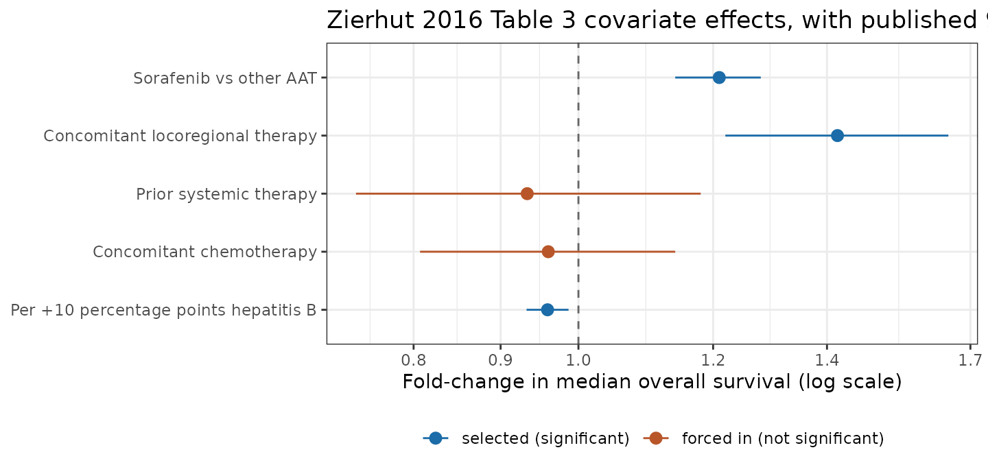
The two forced-in terms straddle 1.0, exactly as the paper says: “the 95% confidence intervals of their estimates spanned both beneficial and detrimental effects.”
4. The between-study random effect cancels within a trial
gamma_j is a study-level draw shared by
every arm of the same trial. That structure is load-bearing, and it is
what makes the paper’s “true” mOS ratio so much tighter (0.774 to 0.891)
than the distribution of either arm’s mOS on its own: within one
simulated trial, gamma_j appears identically in both arms
and cancels exactly from the ratio.
Encoding that in rxode2 means one id per
trial, with one observation record per
arm. The records are distinguished by
time, which here is a bare arm index and carries no
elapsed-time meaning - the model has no time axis at all.
n_trials <- 200  # simulated trials, not patients

paired <- do.call(rbind, lapply(seq_len(n_trials), function(i) {
  data.frame(
    id = i, time = c(0, 1), evid = 0, amt = NA_real_,
    ON_TREATMENT = c(0, 1), SORAFENIB = 0, CONMED_LOCOREGIONAL = 0,
    DIS_CHB_PERCENT = 50, PRIOR_SYSTEMIC = 1, CONMED_CHEMO = 0
  )
}))

rxode2::rxSetSeed(20160515)
# zeroRe(..., "sigma") keeps the between-study effect and drops the
# residual, which the source scales per record by each arm's own
# published standard error (see Errata).
sim_trials <- rxSolve(rxode2::zeroRe(mod, "sigma"), paired, returnType = "data.frame")
#> ℹ parameter labels from comments will be replaced by 'label()'

wide <- sim_trials |>
  dplyr::select(id, time, mos) |>
  tidyr::pivot_wider(names_from = time, values_from = mos, names_prefix = "arm") |>
  dplyr::mutate(ratio = arm0 / arm1)

ratio_spread <- diff(range(wide$ratio))
xi_recovered <- sd(log(wide$arm1))
The ratio is identical in every one of the 200 simulated trials -
0.831567, against the closed-form
exp(theta_PBO - theta_AAT) of 0.831567 - while the arms
themselves vary substantially across trials.
stopifnot(
  # Exact cancellation: gamma_j is shared within a trial, so the ratio
  # carries no between-study variance whatsoever. This is a structural
  # identity, not a statistical one, so the bound is at solver precision.
  ratio_spread < 1e-8,
  abs(unique(round(wide$ratio, 10))[1] - exp(th[["lmos_pbo"]] - th[["lmos_aat"]])) < 1e-8,

  # Recovery of xi from the simulated cohort. The band is the Monte Carlo
  # standard error of a sample SD at n = 200, xi / sqrt(2 * (n - 1)) =
  # 0.0108, widened to 4 SE so a different rxode2 RNG stream (CI resolves
  # a different rxode2 build, and the draw is not portable across solver
  # thread counts) cannot flip it.
  abs(xi_recovered - 0.216) < 4 * 0.216 / sqrt(2 * (n_trials - 1))
)
sim_trials |>
  dplyr::mutate(arm = ifelse(time == 0, "BSC + placebo", "BSC + non-sorafenib AAT")) |>
  ggplot(aes(x = mos, fill = arm)) +
  geom_density(alpha = 0.45, colour = NA) +
  geom_vline(
    data = data.frame(x = mos_by_arm[1:2],
                      arm = c("BSC + placebo", "BSC + non-sorafenib AAT")),
    aes(xintercept = x, colour = arm), linetype = "dashed", show.legend = FALSE
  ) +
  scale_fill_manual(values = c("BSC + placebo" = "#b8562a",
                               "BSC + non-sorafenib AAT" = "#1b6ca8"), name = NULL) +
  scale_colour_manual(values = c("BSC + placebo" = "#b8562a",
                                 "BSC + non-sorafenib AAT" = "#1b6ca8")) +
  labs(
    x = "Simulated trial-arm median overall survival (months)",
    y = "Density",
    title = "Between-study variability in the NCT01210495 simulation population",
    subtitle = paste0(
      "Structurally comparable to Zierhut 2016 Figure 3a; dashed lines are the ",
      "published typical values.\nBetween-study effect only - the residual and ",
      "parameter uncertainty of the paper's own simulation are not included."
    )
  ) +
  theme_bw() +
  theme(legend.position = "bottom")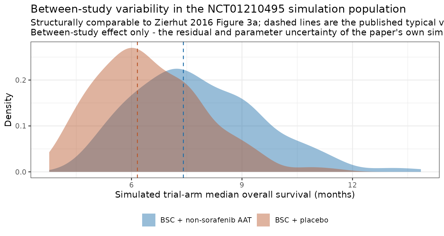
This reproduces the structure of Figure 3a but deliberately not its width: the published distribution also carries parameter-estimate uncertainty (drawn from the Hessian) and the per-arm-size residual, neither of which travels with a packaged model. See Errata.
5. Covariate response surface
The hepatitis B slope is the only continuous effect in the model, and it is the one most likely to be mis-signed or mis-scaled in transcription (a fraction-versus-percent slip would be a 100-fold error). Sweeping it across the observed 4.8% to 100% range, for each combination of the binary indicators, shows both the sign and the magnitude directly.
grid <- tidyr::expand_grid(
  DIS_CHB_PERCENT = seq(5, 100, by = 1),
  scenario = c("Placebo", "Other AAT", "Sorafenib", "Sorafenib + locoregional")
) |>
  dplyr::mutate(
    ON_TREATMENT        = as.numeric(scenario != "Placebo"),
    SORAFENIB           = as.numeric(scenario %in% c("Sorafenib", "Sorafenib + locoregional")),
    CONMED_LOCOREGIONAL = as.numeric(scenario == "Sorafenib + locoregional"),
    PRIOR_SYSTEMIC      = 0,
    CONMED_CHEMO        = 0,
    id                  = dplyr::row_number(),
    time                = 0,
    evid                = 0,
    amt                 = NA_real_
  )

surface <- rxSolve(
  rxode2::zeroRe(mod),
  as.data.frame(grid[, setdiff(names(grid), "scenario")]),
  returnType = "data.frame"
)
#> ℹ parameter labels from comments will be replaced by 'label()'
#> ℹ omega/sigma items treated as zero: 'eta_study_lnmos'
#> Warning: multi-subject simulation without without 'omega'
surface$scenario <- grid$scenario[match(surface$id, grid$id)]

ggplot(surface, aes(x = DIS_CHB_PERCENT, y = mos, colour = scenario)) +
  geom_line(linewidth = 0.9) +
  geom_vline(xintercept = 34, linetype = "dotted", colour = "grey30") +
  annotate("text", x = 34, y = max(surface$mos), hjust = -0.05, vjust = 1,
           label = "analysis-set median, 34%", size = 3, colour = "grey30") +
  labs(
    x = "Hepatitis B positive patients in the trial arm (%)",
    y = "Typical median overall survival (months)",
    colour = NULL,
    title = "Typical-value response surface, treatment-naive population",
    subtitle = "Every curve is the paper's own parameterisation; no eta or residual is drawn."
  ) +
  theme_bw() +
  theme(legend.position = "bottom")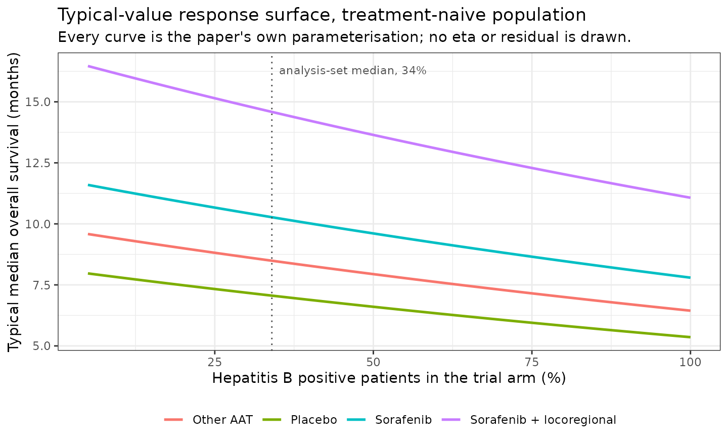
# The slope must be negative everywhere and must deliver exactly the
# published per-percentage-point effect. Comparing the arm-type curves to
# each other also confirms the covariate effects are multiplicative
# (constant ratio across the whole hepatitis B range) rather than
# additive, which is the substance of the source's statement that
# "the additive covariates were interpreted as proportional to mOS".
by_scen <- split(surface[order(surface$DIS_CHB_PERCENT), ], surface$scenario[order(surface$DIS_CHB_PERCENT)])
per_point <- sapply(by_scen, function(d) exp(mean(diff(log(d$mos)))) - 1)
sor_over_aat <- by_scen[["Sorafenib"]]$mos / by_scen[["Other AAT"]]$mos
loc_over_sor <- by_scen[["Sorafenib + locoregional"]]$mos / by_scen[["Sorafenib"]]$mos

stopifnot(
  all(per_point < 0),
  max(abs(per_point - (exp(-0.00418) - 1))) < 1e-8,
  diff(range(sor_over_aat)) < 1e-8, abs(mean(sor_over_aat) - 1.21) < 1e-6,
  diff(range(loc_over_sor)) < 1e-8, abs(mean(loc_over_sor) - 1.42) < 1e-6
)
The full sweep spans 5.36 to 16.47 months, against an observed range across the 68 published arms of 4.2 to 20.8 months - so the model’s covariate space covers the data it was fitted to, without the covariate effects being large enough to reach the extremes on their own (which is what the between-study term and the arms’ own residuals supply).
Assumptions and deviations
-
The residual is encoded at unit study weight.
Zierhut 2016 scales the residual by each arm’s own reported standard
error of
ln(mOS)(eps_ij * SE_ij) and fixes the unit-weight SD at 1, because an estimated value below 1 would mean the model was less variable than the published arms themselves. That per-arm standard error is a property of each published trial, not of the model, so it has noini()home - the packaged model carriesexpSd = fixed(1)and the scaling must be supplied downstream. A bare stochasticrxSolve()therefore applies a residual about five-fold too wide: the per-arm SE had median 0.183 across the analysis set (Table 2), so the unit-weight draw is roughly1 / 0.183times too large at the median arm. Every simulation in this vignette usesrxode2::zeroRe(mod, "sigma")or fullzeroRe()for that reason. This follows the convention of the library’s other MBMA extractions (see theN_ARMentry ininst/references/covariate-columns.md, which blesses the unweighted encoding where the arm weight touches only the residual). - Parameter-estimate uncertainty is not carried. The paper’s simulations draw the fixed effects from the Hessian-derived covariance matrix; the packaged model carries point estimates only, and the source publishes marginal 95% CIs but no covariance matrix. The simulated distributions here are therefore narrower than Figure 3’s, and the reproduction targets are the typical values and the “true” ratios, which are unaffected.
-
AAT and PBO are carried as one column, not two. The
source’s equation has separate
AATandPBOindicators, but its own text states they are “mutually exclusive and collectively exhaustive”. The model consumesON_TREATMENTand computes the placebo indicator as1 - ON_TREATMENT, which is algebraically identical and makes the exhaustiveness structural - an input row cannot set both to 1 and silently sum two intercepts. -
timeis an arm index, not a time. The model has no time axis. Where a simulation puts two records under oneid(to share a between-study draw across a trial’s arms),timeonly distinguishes the records. -
Prior systemic therapy is all-or-nothing at the arm
level. The binary
PRIOR_SYSTEMICis 1 only for the 7 arms whose entire population was pretreated. The 18 arms of mixed treatment line take 0, so this column is not the complement of a first-line indicator, and the continuous “percent with prior systemic tx” of Table 2 is not what the model consumes. -
No individual-level interpretation is available.
Covariate relationships estimated on trial-arm aggregates need not hold
within patients (the ecological-inference problem), which the paper
lists as its first limitation.
DIS_CHB_PERCENTin particular is an arm composition, and the fitted slope is a property of trials, not a statement that an individual hepatitis-B-positive patient survives 0.4% less long. - Locoregional therapy means concomitant, not prior. The model carries no prior-locoregional covariate, which is a real gap in aHCC where prior transarterial chemoembolization is common. The 42% effect also rests on only 7 arms.
Errata and source observations
-
Table 2’s arithmetic mean mOS of 6.6 months is not
reproducible and is treated here as a typographical error. With
68 arms, a minimum of 4.2 months and a median of 9.4 months, the
arithmetic mean cannot fall below
(9.4 + 4.2) / 2 = 6.8months. The paper’s ownln(mOS)row (mean 2.18, SD 0.36) implies an arithmetic mean ofexp(2.18 + 0.36^2 / 2) = 9.4months. The median and range are internally consistent with that row -exp(2.24) = 9.4,exp(1.44) = 4.2,exp(3.04) = 20.9- so only the mean cell is affected. No model parameter depends on it; it appears in the packagedpopulationmetadata with this note attached. -
No erratum or corrigendum was found for this
article. CPT:PSP lists none against the DOI, and the paper has been in
print since May
- The “other AAT” class is heterogeneous by construction. 36 of the 68 arms pool 14 different agents at 1 to 9 arms each, and the model gives them a single shared intercept with sorafenib as the only named exception. A prediction for a specific non-sorafenib agent inherits that pooling.
- Asian study site was investigated but not encodable. After the axitinib trial reported a site effect, the authors re-examined Asian geography as a placebo-arm-specific covariate post hoc. It showed a trend only (change in objective function -2.63, against the 3.84 entry threshold), and the Discussion reports the implied mOS ratios (0.821 Asian, 0.902 non-Asian) without a fitted coefficient - so there is no value to encode. The same applies to publication year (-0.449), which the Discussion argues is the most likely explanation for the phase II trial’s higher observed survival in both arms.
- Supplementary Figure S1 (the literature-screening flow diagram) is the only supplementary material referenced, and it contains no parameter values.
- The trial this model was built to predict did not behave as predicted. NCT01210495 read out afterwards with 12.7 months on axitinib against 9.7 on placebo (HR 0.870, p = 0.211) - both arms well above the simulated 7.40 and 6.16. The simulated ratio nonetheless bracketed the observed hazard ratio. The paper’s proposed explanation, improving best supportive care over time, is untested in this dataset. ```