Biologics and small targeted molecules for Crohn's disease: CDAI, CRP and IBDQ MBMA (Yu 2022)
Source:vignettes/articles/Yu_2022_crohns_mbma.Rmd
Yu_2022_crohns_mbma.RmdModel and source
Yu B, Zhao L, Jin S, He H, Zhang J, Wang X. Model-Based Meta-Analysis on the Efficacy of Biologics and Small Targeted Molecules for Crohn’s Disease. Front Immunol. 2022;13:828219. doi:10.3389/fimmu.2022.828219.
Yu 2022 is a model-based meta-analysis (MBMA) of 24 biologics and small targeted molecules in moderate-to-severe Crohn’s disease, built from 46 double-blind randomised trials (induction period only). It fits six independent models, one per end point, and this package ships each as its own model file:
| Model file | End point | Output | Trials |
|---|---|---|---|
Yu_2022_crohns_cdai150_mbma |
clinical remission, CDAI < 150 | prob_cdai150 |
38 |
Yu_2022_crohns_cdai100_mbma |
clinical response, CDAI reduction >= 100 | prob_cdai100 |
27 |
Yu_2022_crohns_cdai70_mbma |
clinical response, CDAI reduction >= 70 | prob_cdai70 |
24 |
Yu_2022_crohns_dcdai_mbma |
change from baseline in CDAI | d_cdai |
21 |
Yu_2022_crohns_dcrp_mbma |
change from baseline in CRP | d_crp |
26 |
Yu_2022_crohns_dibdq_mbma |
change from baseline in IBDQ | d_ibdq |
20 |
Every model has the same structure. The outcome of a trial arm is a placebo term plus one drug term; the three responder rates are modelled on the logit scale and the three changes from baseline on their natural scale. Each drug has its own maximum effect, which is a constant, a linear function of dose, or an Emax function of dose. The JAK-inhibitor effects in the CDAI150 model, and every drug effect in the Delta CDAI model, switch on exponentially over time. The arm’s baseline characteristics multiply every drug effect through a power function of the covariate over its dataset mean.
modNames <- c(
  cdai150 = "Yu_2022_crohns_cdai150_mbma", cdai100 = "Yu_2022_crohns_cdai100_mbma",
  cdai70 = "Yu_2022_crohns_cdai70_mbma", dcdai = "Yu_2022_crohns_dcdai_mbma",
  dcrp = "Yu_2022_crohns_dcrp_mbma", dibdq = "Yu_2022_crohns_dibdq_mbma"
)
outNames <- c(
  cdai150 = "prob_cdai150", cdai100 = "prob_cdai100", cdai70 = "prob_cdai70",
  dcdai = "d_cdai", dcrp = "d_crp", dibdq = "d_ibdq"
)
uis <- lapply(modNames, function(nm) rxode2::rxode2(readModelDb(nm)))
Population
All six models operate at the study-arm level: one observation is one trial arm’s responder proportion or mean change at one visit, not one patient’s outcome. The source identified 46 trials, 146 treatment arms and 12,846 patients from MEDLINE, CENTRAL, EMBASE and ClinicalTrials.gov to 14 March 2020 (Methods ‘Data Development’; Results ‘Available Data’). Patients were adults with moderate-to-severe active Crohn’s disease; concomitant 5-ASA, oral steroids and immunomodulators and prior TNF-inhibitor exposure were allowed. Table 1 gives the overall means: 46.09% men, age 37.20 years, disease duration 9.52 years, baseline CDAI 306.75, baseline CRP 1.67 and baseline IBDQ 127.37.
pop <- readModelDb(modNames[["cdai150"]])()$population
tibble::tibble(
  Field = c("Species", "Trials", "Patients", "Female (%)", "Age", "Disease state"),
  Value = c(
    pop$species, pop$n_studies, pop$n_subjects, pop$sex_female_pct,
    pop$age_range, pop$disease_state
  )
) |>
knitr::kable()| Field | Value |
|---|---|
| Species | human |
| Trials | 46 |
| Patients | 12846 |
| Female (%) | 53.91 |
| Age | adults (>= 18 years); per-drug arm-mean ages 34.8-41.0 years (Table 1; overall mean 37.2) |
| Disease state | moderate-to-severe active Crohn’s disease confirmed by radiologic, endoscopic or histologic criteria; induction-period data only; prior TNF-inhibitor exposure and concomitant 5-ASA, oral steroids and immunomodulators allowed. Table 1 overall means: disease duration 9.52 years, baseline CDAI 306.75, baseline CRP 1.67, baseline IBDQ 127.37 |
Source trace
The display equations of the main text are images in the published
PDF. The Supplementary Materials (DataSheet 2) restate them as text and
also print the authors’ R code (nlme::gnls) for each final
model. That code is treated as the authority wherever the two differ.
The analysis dataset is Supplementary DataSheet 1. Every
ini() value carries its own trace in the model files.
tibble::tribble(
  ~Component, ~Source,
  "P = expit(E0 + Edrug) for CDAI150, CDAI-100, CDAI-70", "DataSheet 2 Equations 9-10; model code 'yp = exp(emax)/(1+exp(emax))'",
  "Y = E0 + Edrug for Delta CDAI, Delta CRP, Delta IBDQ", "DataSheet 2 Equation 7; model code",
  "E0 estimated separately for every trial and visit", "Methods 'Model Development'; model code 'eo ~ -1 + I(group.week)'",
  "Edrug = Emax * (1 - exp(-k * t))", "DataSheet 2 Equation 3; code writes the rate as exp(k)",
  "Emax constant, slope * DOSE, or Emax * DOSE / (DOSE + ED50)", "Supplementary Table 2-7 footnotes a, b; code",
  "Covariate effect = (X / mean(X))^theta on every drug effect", "DataSheet 2 Equation 12; code 'emrel'",
  "Residual weight sqrt(P * (1 - P) / N) or SD / sqrt(N)", "DataSheet 2 Equations 8 and 11; code 'weights ='"
) |>
knitr::kable(caption = "Structural, covariate and residual equations.")| Component | Source |
|---|---|
| P = expit(E0 + Edrug) for CDAI150, CDAI-100, CDAI-70 | DataSheet 2 Equations 9-10; model code ‘yp = exp(emax)/(1+exp(emax))’ |
| Y = E0 + Edrug for Delta CDAI, Delta CRP, Delta IBDQ | DataSheet 2 Equation 7; model code |
| E0 estimated separately for every trial and visit | Methods ‘Model Development’; model code ‘eo ~ -1 + I(group.week)’ |
| Edrug = Emax * (1 - exp(-k * t)) | DataSheet 2 Equation 3; code writes the rate as exp(k) |
| Emax constant, slope * DOSE, or Emax * DOSE / (DOSE + ED50) | Supplementary Table 2-7 footnotes a, b; code |
| Covariate effect = (X / mean(X))^theta on every drug effect | DataSheet 2 Equation 12; code ‘emrel’ |
| Residual weight sqrt(P * (1 - P) / N) or SD / sqrt(N) | DataSheet 2 Equations 8 and 11; code ‘weights =’ |
tibble::tribble(
  ~Model, ~Parameters, ~Source,
  "CDAI150", "22 drug effects, k_JAK, baseline CDAI and CRP exponents", "Supplementary Table 2; key rows in Table 2",
  "CDAI-100", "17 drug effects (adalimumab Emax/ED50), baseline CDAI and CRP exponents", "Supplementary Table 3; key rows in Table 2",
  "CDAI-70", "16 drug effects (upadacitinib Emax/ED50), baseline CDAI and CRP exponents", "Supplementary Table 4; key rows in Table 2",
  "Delta CDAI", "15 drug effects (adalimumab Emax/ED50), k_general, baseline CDAI exponent", "Supplementary Table 5; key rows in Table 2",
  "Delta CRP", "17 drug effects, age, disease duration and baseline CRP exponents", "Supplementary Table 6; key rows in Table 2",
  "Delta IBDQ", "16 drug effects, disease duration exponent", "Supplementary Table 7; key rows in Table 2",
  "all", "placebo response at the typical trial, Week 12", "Results 'Model Simulation'",
  "all", "covariate reference values (dataset means)", "Supplementary DataSheet 1",
  "CDAI150, CDAI-100, CDAI-70", "residual multiplier on the binomial SE", "not reported; the maintainers' refit (see Assumptions)"
) |>
knitr::kable(caption = "Parameter provenance by block.")| Model | Parameters | Source |
|---|---|---|
| CDAI150 | 22 drug effects, k_JAK, baseline CDAI and CRP exponents | Supplementary Table 2; key rows in Table 2 |
| CDAI-100 | 17 drug effects (adalimumab Emax/ED50), baseline CDAI and CRP exponents | Supplementary Table 3; key rows in Table 2 |
| CDAI-70 | 16 drug effects (upadacitinib Emax/ED50), baseline CDAI and CRP exponents | Supplementary Table 4; key rows in Table 2 |
| Delta CDAI | 15 drug effects (adalimumab Emax/ED50), k_general, baseline CDAI exponent | Supplementary Table 5; key rows in Table 2 |
| Delta CRP | 17 drug effects, age, disease duration and baseline CRP exponents | Supplementary Table 6; key rows in Table 2 |
| Delta IBDQ | 16 drug effects, disease duration exponent | Supplementary Table 7; key rows in Table 2 |
| all | placebo response at the typical trial, Week 12 | Results ‘Model Simulation’ |
| all | covariate reference values (dataset means) | Supplementary DataSheet 1 |
| CDAI150, CDAI-100, CDAI-70 | residual multiplier on the binomial SE | not reported; the maintainers’ refit (see Assumptions) |
Regimens
Each drug enters through its own
CONMED_<drug>_DOSE column; an arm sets the column of
the drug it received and leaves every other column at 0, so a placebo
arm reduces to the placebo term. The value is the DOSE
column of the deposited dataset: weight-based regimens are in mg at 70
kg, adalimumab is the week-0 induction dose, and the JAK inhibitors are
the dose per administration of their twice-daily regimen. Only the
dose-response drugs read the magnitude; for every other drug only
> 0 matters. The regimens below are the rows of the
paper’s Week-12 ranking figures (Figures 4 and 5).
# Figure row label -> covariate column and the dataset DOSE value it maps to.
regimen <- tibble::tribble(
  ~lab,               ~col,                          ~dose,
  "infliximab",       "CONMED_INFLIXIMAB_DOSE",        350,
  "natalizumab",      "CONMED_NATALIZUMAB_DOSE",       300,
  "cdp571",           "CONMED_CDP571_DOSE",            700,
  "etanercept",       "CONMED_ETANERCEPT_DOSE",         25,
  "certolizumab",     "CONMED_CERTOLIZUMAB_DOSE",      400,
  "certolizumab_400", "CONMED_CERTOLIZUMAB_DOSE",      400,
  "certolizumab_200", "CONMED_CERTOLIZUMAB_DOSE",      200,
  "certolizumab_100", "CONMED_CERTOLIZUMAB_DOSE",      100,
  "adalimumab",       "CONMED_ADALIMUMAB_DOSE",        160,
  "adalimumab_160",   "CONMED_ADALIMUMAB_DOSE",        160,
  "adalimumab_80",    "CONMED_ADALIMUMAB_DOSE",         80,
  "adalimumab_40",    "CONMED_ADALIMUMAB_DOSE",         40,
  "onercept",         "CONMED_ONERCEPT_DOSE",           50,
  "semapimod",        "CONMED_SEMAPIMOD_DOSE",         180,
  "vedolizumab",      "CONMED_VEDOLIZUMAB_DOSE",       300,
  "abrilumab",        "CONMED_ABRILUMAB_DOSE",         210,
  "ustekinumab",      "CONMED_USTEKINUMAB_DOSE",        90,
  "apilimod",         "CONMED_APILIMOD_DOSE",          100,
  "risankizumab",     "CONMED_RISANKIZUMAB_DOSE",      600,
  "risankizumab_600", "CONMED_RISANKIZUMAB_DOSE",      600,
  "risankizumab_200", "CONMED_RISANKIZUMAB_DOSE",      200,
  "brazikumab",       "CONMED_BRAZIKUMAB_DOSE",        700,
  "pf04236921",       "CONMED_PF04236921_DOSE",        200,
  "pf04236921_200",   "CONMED_PF04236921_DOSE",        200,
  "pf04236921_50",    "CONMED_PF04236921_DOSE",         50,
  "pf04236921_10",    "CONMED_PF04236921_DOSE",         10,
  "andecaliximab",    "CONMED_ANDECALIXIMAB_DOSE",     300,
  "tofacitinib",      "CONMED_TOFACITINIB_DOSE",        10,
  "filgotinib",       "CONMED_FILGOTINIB_DOSE",        200,
  "upadacitinib",     "CONMED_UPADACITINIB_DOSE",       24,
  "upadacitinib_24",  "CONMED_UPADACITINIB_DOSE",       24,
  "upadacitinib_12",  "CONMED_UPADACITINIB_DOSE",       12,
  "upadacitinib_6",   "CONMED_UPADACITINIB_DOSE",        6,
  "upadacitinib_3",   "CONMED_UPADACITINIB_DOSE",        3,
  "laquinimod",       "CONMED_LAQUINIMOD_DOSE",          2,
  "abatacept",        "CONMED_ABATACEPT_DOSE",         700,
  "ontamalimab",      "CONMED_ONTAMALIMAB_DOSE",        75,
  "fontolizumab",     "CONMED_FONTOLIZUMAB_DOSE",      280,
  "vercirnon",        "CONMED_VERCIRNON_DOSE",         500
)

# The typical trial of Results 'Model Simulation': baseline CDAI 306.75,
# baseline CRP 1.67, disease duration 9.52 years. The paper does not state the
# age of that trial; the Table 1 overall mean, 37.20 years, is used.
typicalTrial <- list(SCORE_CDAI = 306.75, CRP = 1.67, T_DIAG_CD = 9.52, AGE = 37.20)

#' Build an rxode2 input frame with one id per row of `arms` (columns lab, col,
#' dose), observed at `times`, for the model `ui`. Every covariate column the
#' model declares is created; the drug columns are 0 except the arm's own.
makeArmData <- function(ui, arms, times, cov = typicalTrial, nArm = 100) {
  cd <- names(ui$meta$covariateData)
  do.call(rbind, lapply(seq_len(nrow(arms)), function(i) {
    d <- data.frame(id = i, time = times, N_ARM = nArm)
    for (cc in cd[cd != "N_ARM"]) d[[cc]] <- if (cc %in% names(cov)) cov[[cc]] else 0
    if (!is.na(arms$col[i])) d[[arms$col[i]]] <- arms$dose[i]
    d
  }))
}

#' Typical-value (no residual) solve of `ui` for `arms`; returns one row per
#' arm and time with the arm label attached.
solveArms <- function(ui, arms, times, ...) {
  sol <- rxode2::rxSolve(rxode2::zeroRe(ui, "sigma"), makeArmData(ui, arms, times, ...),
                         returnType = "data.frame")
  # rxode2 drops the id column when only one id is solved.
  if (is.null(sol$id)) sol$id <- 1L
  mutate(sol, lab = arms$lab[as.integer(id)])
}
Reproducing Figures 4 and 5 (Week-12 ranking)
Figures 4 and 5 rank every regimen by its predicted Week-12 outcome in the typical trial, with the simulated placebo response drawn as a dashed line. Despite the caption’s “placebo-corrected”, the plotted values are absolute: the dashed placebo lines sit at the placebo values quoted in the Results (21.26%, 31.28%, 39.48%, -58.67, 0.016 and 17.36), and the quoted regimen values (for example PF-04236921 200 mg, 56.12% in CDAI150) read directly off the axis. The maintainers digitised every point from the figure rasters; the digitisation reproduces each value quoted in the Results text to within 0.1 unit.
These values are predictions, not parameter estimates, so reproducing them is an independent check on the whole encoding: 128 regimen points across six panels.
# Digitised by the maintainers from Figures 4A-C and 5A-C (Week 12, typical
# trial); percent for the three responder rates, points or mg/dL otherwise.
fig <- list(
  cdai150 = tibble::tribble(
    ~lab, ~fig,
    "pf04236921_200", 56.12, "risankizumab_600", 53.52, "infliximab", 44.38,
    "adalimumab_160", 39.80, "laquinimod", 38.19, "fontolizumab", 35.77,
    "filgotinib", 35.56, "vedolizumab", 34.20, "brazikumab", 33.96,
    "upadacitinib", 31.42, "abrilumab", 30.50, "risankizumab_200", 30.47,
    "adalimumab_80", 29.71, "certolizumab", 29.49, "ontamalimab", 29.12,
    "natalizumab", 28.92, "ustekinumab", 28.84, "pf04236921_50", 28.50,
    "tofacitinib", 27.38, "adalimumab_40", 25.28, "cdp571", 24.31,
    "onercept", 24.24, "pf04236921_10", 22.60, "apilimod", 19.55,
    "vercirnon", 18.53, "andecaliximab", 17.48, "etanercept", 12.35
  ),
  cdai100 = tibble::tribble(
    ~lab, ~fig,
    "infliximab", 56.74, "upadacitinib_24", 56.28, "brazikumab", 54.12,
    "adalimumab_160", 46.92, "vedolizumab", 45.95, "tofacitinib", 45.82,
    "natalizumab", 44.68, "adalimumab_80", 44.21, "pf04236921", 43.75,
    "laquinimod", 43.37, "upadacitinib_12", 43.35, "ustekinumab", 43.09,
    "filgotinib", 41.38, "adalimumab_40", 41.19, "certolizumab", 41.14,
    "fontolizumab", 40.66, "upadacitinib_6", 37.12, "ontamalimab", 36.45,
    "vercirnon", 34.49, "upadacitinib_3", 34.15, "onercept", 32.05,
    "apilimod", 24.26
  ),
  cdai70 = tibble::tribble(
    ~lab, ~fig,
    "infliximab", 67.47, "adalimumab", 60.31, "pf04236921", 56.57,
    "upadacitinib_24", 55.08, "upadacitinib_12", 52.52, "certolizumab", 51.01,
    "natalizumab", 50.80, "upadacitinib_6", 49.64, "cdp571", 49.12,
    "laquinimod", 48.10, "vedolizumab", 47.44, "tofacitinib", 47.00,
    "etanercept", 46.84, "upadacitinib_3", 46.70, "vercirnon", 45.62,
    "brazikumab", 44.86, "ustekinumab", 44.71, "ontamalimab", 41.99,
    "semapimod", 40.33
  ),
  dcdai = tibble::tribble(
    ~lab, ~fig,
    "risankizumab", -133.43, "adalimumab_160", -124.75, "natalizumab", -105.61,
    "adalimumab_80", -104.57, "fontolizumab", -96.24, "brazikumab", -95.41,
    "abrilumab", -91.27, "filgotinib", -88.20, "adalimumab_40", -87.77,
    "certolizumab", -87.56, "pf04236921", -87.16, "tofacitinib", -82.89,
    "vedolizumab", -79.34, "abatacept", -76.95, "cdp571", -75.53,
    "vercirnon", -74.87, "etanercept", -73.22
  ),
  dcrp = tibble::tribble(
    ~lab, ~fig,
    "pf04236921_200", -5.503, "pf04236921_50", -2.673, "natalizumab", -0.939,
    "pf04236921_10", -0.707, "infliximab", -0.638, "adalimumab", -0.483,
    "certolizumab_400", -0.462, "certolizumab_200", -0.214, "ustekinumab", -0.213,
    "upadacitinib_24", -0.173, "cdp571", -0.135, "fontolizumab", -0.110,
    "certolizumab_100", -0.095, "upadacitinib_12", -0.072, "semapimod", -0.057,
    "tofacitinib", -0.062, "ontamalimab", -0.035, "upadacitinib_6", -0.032,
    "upadacitinib_3", 0.001, "risankizumab", 0.021, "vedolizumab", 0.073,
    "vercirnon", 0.139, "laquinimod", 0.301, "abatacept", 0.678
  ),
  dibdq = tibble::tribble(
    ~lab, ~fig,
    "tofacitinib", 70.12, "risankizumab_600", 50.13, "infliximab", 32.99,
    "adalimumab_160", 32.89, "risankizumab_200", 28.30, "adalimumab_80", 25.12,
    "filgotinib", 24.11, "upadacitinib", 22.10, "cdp571", 21.29,
    "adalimumab_40", 21.24, "vercirnon", 20.82, "natalizumab", 20.07,
    "vedolizumab", 18.36, "certolizumab", 17.49, "fontolizumab", 16.74,
    "semapimod", 16.04, "etanercept", 15.75, "abatacept", 13.83,
    "apilimod", 9.04
  )
)
placebo <- c(cdai150 = 21.26, cdai100 = 31.28, cdai70 = 39.48,
             dcdai = -58.67, dcrp = 0.016, dibdq = 17.36)
binary <- c(cdai150 = TRUE, cdai100 = TRUE, cdai70 = TRUE,
            dcdai = FALSE, dcrp = FALSE, dibdq = FALSE)
# Deterministic typical-value solves: rxode2 warns that there is no omega and,
# after zeroRe(), no sigma, which is expected here.
cmp <- bind_rows(lapply(names(fig), function(k) {
  arms <- left_join(fig[[k]], regimen, by = "lab")
  sol <- solveArms(uis[[k]], arms, times = 12)
  scale <- if (binary[[k]]) 100 else 1
  arms |>
    mutate(
      endpoint = k,
      model = scale * sol[[outNames[[k]]]],
      covEff = sol$covEff,
      diff = model - fig
    )
}))
stopifnot(nrow(cmp) == 128, !anyNA(cmp$model))
Most of the 128 points are reproduced closely. A few groups of points are not, and each departure has a known cause. The published values are medians of 10,000 simulations that sample the parameters from their uncertainty. For a constant or linear drug effect, that median equals the typical-value prediction. When the effect is a nonlinear function of poorly identified parameters, it does not. Those points are flagged here and checked separately in the next section:
- the JAK inhibitors in CDAI150, whose effect multiplies an onset rate with a 95% CI spanning two orders of magnitude (0.01-1.40 /week);
- the adalimumab Emax/ED50 dose-responses in CDAI-100 and Delta CDAI and the upadacitinib Emax/ED50 dose-response in CDAI-70, whose ED50 intervals are also that wide;
- upadacitinib in Delta CRP, whose slope was itself back-solved from Figure 5B (see Assumptions), so it is not an independent check.
flagged <- tibble::tribble(
  ~endpoint, ~lab,
  "cdai150", "tofacitinib", "cdai150", "filgotinib", "cdai150", "upadacitinib",
  "cdai100", "adalimumab_160", "cdai100", "adalimumab_80", "cdai100", "adalimumab_40",
  "cdai70", "upadacitinib_24", "cdai70", "upadacitinib_12", "cdai70", "upadacitinib_6",
  "cdai70", "upadacitinib_3",
  "dcdai", "adalimumab_160", "dcdai", "adalimumab_80", "dcdai", "adalimumab_40",
  "dcrp", "upadacitinib_24", "dcrp", "upadacitinib_12", "dcrp", "upadacitinib_6",
  "dcrp", "upadacitinib_3"
) |>
  mutate(flag = TRUE)
cmp <- cmp |>
  left_join(flagged, by = c("endpoint", "lab")) |>
  mutate(flag = !is.na(flag))

cmp |>
  mutate(Regimen = ifelse(flag, paste0(lab, " *"), lab)) |>
  select(endpoint, Regimen, fig, model, diff) |>
  rename(`End point` = endpoint, `Figure 4/5` = fig, `Model (typical)` = model,
         `Model - figure` = diff) |>
  knitr::kable(digits = 2, caption = paste(
    "Week-12 typical-trial prediction against the digitised Figures 4 and 5",
    "(percent for the responder rates; * = nonlinear-uncertainty or",
    "back-solved point, see text)."
))| End point | Regimen | Figure 4/5 | Model (typical) | Model - figure |
|---|---|---|---|---|
| cdai150 | pf04236921_200 | 56.12 | 56.21 | 0.09 |
| cdai150 | risankizumab_600 | 53.52 | 53.06 | -0.46 |
| cdai150 | infliximab | 44.38 | 44.43 | 0.05 |
| cdai150 | adalimumab_160 | 39.80 | 39.87 | 0.07 |
| cdai150 | laquinimod | 38.19 | 38.09 | -0.10 |
| cdai150 | fontolizumab | 35.77 | 35.91 | 0.14 |
| cdai150 | filgotinib * | 35.56 | 43.03 | 7.47 |
| cdai150 | vedolizumab | 34.20 | 34.20 | 0.00 |
| cdai150 | brazikumab | 33.96 | 33.99 | 0.03 |
| cdai150 | upadacitinib * | 31.42 | 36.31 | 4.89 |
| cdai150 | abrilumab | 30.50 | 30.32 | -0.18 |
| cdai150 | risankizumab_200 | 30.47 | 30.32 | -0.15 |
| cdai150 | adalimumab_80 | 29.71 | 29.73 | 0.02 |
| cdai150 | certolizumab | 29.49 | 29.54 | 0.05 |
| cdai150 | ontamalimab | 29.12 | 29.15 | 0.03 |
| cdai150 | natalizumab | 28.92 | 28.96 | 0.04 |
| cdai150 | ustekinumab | 28.84 | 28.96 | 0.12 |
| cdai150 | pf04236921_50 | 28.50 | 28.50 | 0.00 |
| cdai150 | tofacitinib * | 27.38 | 31.26 | 3.88 |
| cdai150 | adalimumab_40 | 25.28 | 25.26 | -0.02 |
| cdai150 | cdp571 | 24.31 | 24.22 | -0.09 |
| cdai150 | onercept | 24.24 | 24.22 | -0.02 |
| cdai150 | pf04236921_10 | 22.60 | 22.59 | -0.01 |
| cdai150 | apilimod | 19.55 | 19.44 | -0.11 |
| cdai150 | vercirnon | 18.53 | 18.44 | -0.09 |
| cdai150 | andecaliximab | 17.48 | 17.47 | -0.01 |
| cdai150 | etanercept | 12.35 | 12.30 | -0.05 |
| cdai100 | infliximab | 56.74 | 56.45 | -0.29 |
| cdai100 | upadacitinib_24 | 56.28 | 56.24 | -0.04 |
| cdai100 | brazikumab | 54.12 | 53.98 | -0.14 |
| cdai100 | adalimumab_160 * | 46.92 | 49.42 | 2.50 |
| cdai100 | vedolizumab | 45.95 | 45.78 | -0.17 |
| cdai100 | tofacitinib | 45.82 | 45.53 | -0.29 |
| cdai100 | natalizumab | 44.68 | 44.55 | -0.13 |
| cdai100 | adalimumab_80 * | 44.21 | 46.57 | 2.36 |
| cdai100 | pf04236921 | 43.75 | 43.56 | -0.19 |
| cdai100 | laquinimod | 43.37 | 43.07 | -0.30 |
| cdai100 | upadacitinib_12 | 43.35 | 43.34 | -0.01 |
| cdai100 | ustekinumab | 43.09 | 43.07 | -0.02 |
| cdai100 | filgotinib | 41.38 | 41.37 | -0.01 |
| cdai100 | adalimumab_40 * | 41.19 | 42.87 | 1.68 |
| cdai100 | certolizumab | 41.14 | 41.13 | -0.01 |
| cdai100 | fontolizumab | 40.66 | 40.41 | -0.25 |
| cdai100 | upadacitinib_6 | 37.12 | 37.11 | -0.01 |
| cdai100 | ontamalimab | 36.45 | 36.40 | -0.05 |
| cdai100 | vercirnon | 34.49 | 34.58 | 0.09 |
| cdai100 | upadacitinib_3 | 34.15 | 34.13 | -0.02 |
| cdai100 | onercept | 32.05 | 32.14 | 0.09 |
| cdai100 | apilimod | 24.26 | 24.31 | 0.05 |
| cdai70 | infliximab | 67.47 | 67.58 | 0.11 |
| cdai70 | adalimumab | 60.31 | 60.23 | -0.08 |
| cdai70 | pf04236921 | 56.57 | 56.47 | -0.10 |
| cdai70 | upadacitinib_24 * | 55.08 | 57.78 | 2.70 |
| cdai70 | upadacitinib_12 * | 52.52 | 55.54 | 3.02 |
| cdai70 | certolizumab | 51.01 | 51.18 | 0.17 |
| cdai70 | natalizumab | 50.80 | 50.94 | 0.14 |
| cdai70 | upadacitinib_6 * | 49.64 | 52.36 | 2.72 |
| cdai70 | cdp571 | 49.12 | 49.24 | 0.12 |
| cdai70 | laquinimod | 48.10 | 48.27 | 0.17 |
| cdai70 | vedolizumab | 47.44 | 47.55 | 0.11 |
| cdai70 | tofacitinib | 47.00 | 47.07 | 0.07 |
| cdai70 | etanercept | 46.84 | 46.83 | -0.01 |
| cdai70 | upadacitinib_3 * | 46.70 | 48.67 | 1.97 |
| cdai70 | vercirnon | 45.62 | 45.62 | 0.00 |
| cdai70 | brazikumab | 44.86 | 44.90 | 0.04 |
| cdai70 | ustekinumab | 44.71 | 44.90 | 0.19 |
| cdai70 | ontamalimab | 41.99 | 42.05 | 0.06 |
| cdai70 | semapimod | 40.33 | 40.41 | 0.08 |
| dcdai | risankizumab | -133.43 | -134.44 | -1.01 |
| dcdai | adalimumab_160 * | -124.75 | -140.96 | -16.21 |
| dcdai | natalizumab | -105.61 | -106.22 | -0.61 |
| dcdai | adalimumab_80 * | -104.57 | -116.94 | -12.37 |
| dcdai | fontolizumab | -96.24 | -96.63 | -0.39 |
| dcdai | brazikumab | -95.41 | -95.69 | -0.28 |
| dcdai | abrilumab | -91.27 | -91.65 | -0.38 |
| dcdai | filgotinib | -88.20 | -88.44 | -0.24 |
| dcdai | adalimumab_40 * | -87.77 | -95.46 | -7.69 |
| dcdai | certolizumab | -87.56 | -87.86 | -0.30 |
| dcdai | pf04236921 | -87.16 | -87.47 | -0.31 |
| dcdai | tofacitinib | -82.89 | -82.95 | -0.06 |
| dcdai | vedolizumab | -79.34 | -79.39 | -0.05 |
| dcdai | abatacept | -76.95 | -77.36 | -0.41 |
| dcdai | cdp571 | -75.53 | -75.57 | -0.04 |
| dcdai | vercirnon | -74.87 | -74.98 | -0.11 |
| dcdai | etanercept | -73.22 | -73.42 | -0.20 |
| dcrp | pf04236921_200 | -5.50 | -5.68 | -0.17 |
| dcrp | pf04236921_50 | -2.67 | -2.89 | -0.22 |
| dcrp | natalizumab | -0.94 | -0.98 | -0.04 |
| dcrp | pf04236921_10 | -0.71 | -0.79 | -0.08 |
| dcrp | infliximab | -0.64 | -0.67 | -0.03 |
| dcrp | adalimumab | -0.48 | -0.51 | -0.03 |
| dcrp | certolizumab_400 | -0.46 | -0.49 | -0.02 |
| dcrp | certolizumab_200 | -0.21 | -0.23 | -0.02 |
| dcrp | ustekinumab | -0.21 | -0.23 | -0.02 |
| dcrp | upadacitinib_24 * | -0.17 | -0.18 | -0.01 |
| dcrp | cdp571 | -0.14 | -0.15 | -0.02 |
| dcrp | fontolizumab | -0.11 | -0.13 | -0.02 |
| dcrp | certolizumab_100 | -0.10 | -0.11 | -0.01 |
| dcrp | upadacitinib_12 * | -0.07 | -0.08 | -0.01 |
| dcrp | semapimod | -0.06 | -0.06 | -0.01 |
| dcrp | tofacitinib | -0.06 | -0.06 | 0.00 |
| dcrp | ontamalimab | -0.04 | -0.04 | 0.00 |
| dcrp | upadacitinib_6 * | -0.03 | -0.03 | 0.00 |
| dcrp | upadacitinib_3 * | 0.00 | -0.01 | -0.01 |
| dcrp | risankizumab | 0.02 | 0.01 | -0.01 |
| dcrp | vedolizumab | 0.07 | 0.05 | -0.02 |
| dcrp | vercirnon | 0.14 | 0.13 | -0.01 |
| dcrp | laquinimod | 0.30 | 0.30 | -0.01 |
| dcrp | abatacept | 0.68 | 0.68 | 0.00 |
| dibdq | tofacitinib | 70.12 | 78.56 | 8.44 |
| dibdq | risankizumab_600 | 50.13 | 52.17 | 2.04 |
| dibdq | infliximab | 32.99 | 35.60 | 2.61 |
| dibdq | adalimumab_160 | 32.89 | 35.93 | 3.04 |
| dibdq | risankizumab_200 | 28.30 | 28.96 | 0.66 |
| dibdq | adalimumab_80 | 25.12 | 26.64 | 1.52 |
| dibdq | filgotinib | 24.11 | 25.18 | 1.07 |
| dibdq | upadacitinib | 22.10 | 22.81 | 0.71 |
| dibdq | cdp571 | 21.29 | 21.92 | 0.63 |
| dibdq | adalimumab_40 | 21.24 | 22.00 | 0.76 |
| dibdq | vercirnon | 20.82 | 21.47 | 0.65 |
| dibdq | natalizumab | 20.07 | 20.52 | 0.45 |
| dibdq | vedolizumab | 18.36 | 18.49 | 0.13 |
| dibdq | certolizumab | 17.49 | 17.72 | 0.23 |
| dibdq | fontolizumab | 16.74 | 16.97 | 0.23 |
| dibdq | semapimod | 16.04 | 15.85 | -0.19 |
| dibdq | etanercept | 15.75 | 15.61 | -0.14 |
| dibdq | abatacept | 13.83 | 13.25 | -0.58 |
| dibdq | apilimod | 9.04 | 7.78 | -1.26 |
The unflagged points give a direct read of how well the encoding matches. For the three CDAI responder rates the agreement is within a fraction of a percentage point. For Delta CDAI it is within about one CDAI point. For the two continuous end points with steep covariate exponents, Delta CRP (age -7.69, disease duration 4.95) and Delta IBDQ (disease duration -8.98), the drug effects agree up to a common factor near 1. That factor reflects the covariate reference values: they are dataset means that depend on how missing arm covariates were imputed, and the paper does not state the age of its typical trial (see Assumptions). The gate below therefore checks the responder rates and Delta CDAI on the absolute difference. For Delta CRP and Delta IBDQ it checks the ratio of the placebo-corrected drug effects, which cancels that common factor.
chk <- cmp |>
  filter(!flag) |>
  mutate(
    lpFig = ifelse(binary[endpoint], qlogis(fig / 100), fig),
    lpMod = ifelse(binary[endpoint], qlogis(model / 100), model),
    lpPbo = ifelse(binary[endpoint], qlogis(placebo[endpoint] / 100), placebo[endpoint]),
    ratio = (lpMod - lpPbo) / (lpFig - lpPbo)
  )
#> Warning: There were 3 warnings in `mutate()`.
#> The first warning was:
#> ℹ In argument: `lpFig = ifelse(binary[endpoint], qlogis(fig/100), fig)`.
#> Caused by warning in `qlogis()`:
#> ! NaNs produced
#> ℹ Run `dplyr::last_dplyr_warnings()` to see the 2 remaining warnings.
# Points whose placebo-corrected effect is too small to give a stable ratio
# (under 0.1 mg/dL CRP or 2 IBDQ points) are left out of the ratio.
minEffect <- c(dcrp = 0.1, dibdq = 2)
ratioSummary <- chk |>
  filter(endpoint %in% names(minEffect)) |>
  filter(abs(lpFig - lpPbo) > minEffect[endpoint]) |>
  group_by(endpoint) |>
  summarise(medianRatio = median(ratio), n = n(), .groups = "drop")
knitr::kable(ratioSummary, digits = 3,
caption = "Median ratio of model to figure placebo-corrected drug effect, unflagged points.")| endpoint | medianRatio | n |
|---|---|---|
| dcrp | 1.054 | 15 |
| dibdq | 1.162 | 14 |
# Deterministic comparison: typical-value solves at the published parameters
# against fixed digitised values, so a tight bound is appropriate.
stopifnot(
  max(abs(chk$diff[chk$endpoint %in% c("cdai150", "cdai100", "cdai70")])) < 0.5,
  max(abs(chk$diff[chk$endpoint == "dcdai"])) < 1.5,
  abs(ratioSummary$medianRatio[ratioSummary$endpoint == "dcrp"] - 1) < 0.1,
  abs(ratioSummary$medianRatio[ratioSummary$endpoint == "dibdq"] - 1) < 0.2
)
cmp |>
  ggplot(aes(fig, model, shape = flag)) +
  geom_abline(linetype = 2, colour = "grey50") +
  geom_point() +
  scale_shape_manual(values = c(`FALSE` = 16, `TRUE` = 1), guide = "none") +
  facet_wrap(~endpoint, scales = "free") +
  labs(x = "Figure 4/5 (digitised)", y = "Model, typical trial") +
  theme_bw()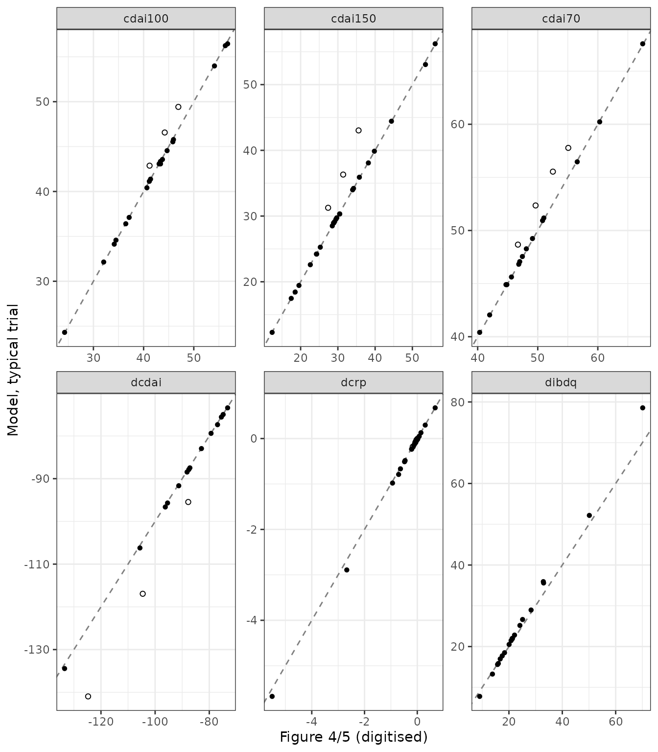
Replicates Figures 4 and 5 of Yu 2022: Week-12 typical-trial prediction (model) against the digitised published points (figure); flagged points are open circles.
Flagged points: parameter uncertainty
The flagged points are checked by repeating the paper’s own procedure: draw the parameters of the nonlinear term from their published 95% confidence intervals and take the median of the resulting prediction. Linear parameters (Emax) are drawn on the natural scale. ED50 and the onset rates are drawn on the log scale, where their published intervals are symmetric. The draws are independent because the paper reports no covariance. The other terms, including the covariate factor, are taken from the model solve. This uses base R’s random number generator, which gives the same stream on every platform.
set.seed(20220317)
nDraw <- 10000
drawN <- function(est, lo, hi) rnorm(nDraw, est, (hi - lo) / 3.92)
drawL <- function(est, lo, hi) exp(rnorm(nDraw, log(est), (log(hi) - log(lo)) / 3.92))
cf <- function(k, lab) cmp$covEff[cmp$endpoint == k & cmp$lab == lab]
pbLogit <- function(k) qlogis(placebo[[k]] / 100)

gJak <- 1 - exp(-drawL(0.11, 0.01, 1.40) * 12)
gAll <- 1 - exp(-drawL(0.22, 0.14, 0.34) * 12)
unc <- bind_rows(
  tibble(endpoint = "cdai150", lab = c("tofacitinib", "filgotinib", "upadacitinib"),
         sim = c(
           100 * median(plogis(pbLogit("cdai150") + drawN(0.76, -1.14, 2.66) * gJak * cf("cdai150", "tofacitinib"))),
           100 * median(plogis(pbLogit("cdai150") + drawN(1.50, -1.02, 4.01) * gJak * cf("cdai150", "filgotinib"))),
           100 * median(plogis(pbLogit("cdai150") + drawN(1.09, -0.39, 2.58) * gJak * cf("cdai150", "upadacitinib")))
         )),
  tibble(endpoint = "cdai100", lab = c("adalimumab_160", "adalimumab_80", "adalimumab_40"),
         dose = c(160, 80, 40)) |>
    rowwise() |>
    mutate(sim = 100 * median(plogis(pbLogit("cdai100") +
      drawN(0.93, 0.30, 1.56) * dose / (dose + drawL(34.13, 1.66, 703.51)) * cf("cdai100", lab)))) |>
    ungroup() |> select(-dose),
  tibble(endpoint = "cdai70", lab = c("upadacitinib_24", "upadacitinib_12", "upadacitinib_6", "upadacitinib_3"),
         dose = c(24, 12, 6, 3)) |>
    rowwise() |>
    mutate(sim = 100 * median(plogis(pbLogit("cdai70") +
      drawN(0.89, 0.09, 1.69) * dose / (dose + drawL(3.91, 0.19, 79.30)) * cf("cdai70", lab)))) |>
    ungroup() |> select(-dose),
  tibble(endpoint = "dcdai", lab = c("adalimumab_160", "adalimumab_80", "adalimumab_40"),
         dose = c(160, 80, 40)) |>
    rowwise() |>
    mutate(sim = median(placebo[["dcdai"]] +
      drawN(-151.24, -322.11, 19.64) * dose / (dose + drawL(112.23, 9.02, 1395.85)) * gAll * cf("dcdai", lab))) |>
    ungroup() |> select(-dose)
)
uncCmp <- unc |>
  left_join(select(cmp, endpoint, lab, fig, model), by = c("endpoint", "lab")) |>
  mutate(errTypical = model - fig, errSim = sim - fig)
uncCmp |>
  rename(`End point` = endpoint, Regimen = lab, Figure = fig,
         `Typical value` = model, `Median over parameter draws` = sim) |>
knitr::kable(digits = 2, caption = "Flagged points: typical value and uncertainty-propagated median against the figure.")| End point | Regimen | Median over parameter draws | Figure | Typical value | errTypical | errSim |
|---|---|---|---|---|---|---|
| cdai150 | tofacitinib | 28.33 | 27.38 | 31.26 | 3.88 | 0.95 |
| cdai150 | filgotinib | 37.15 | 35.56 | 43.03 | 7.47 | 1.59 |
| cdai150 | upadacitinib | 32.50 | 31.42 | 36.31 | 4.89 | 1.08 |
| cdai100 | adalimumab_160 | 47.30 | 46.92 | 49.42 | 2.50 | 0.38 |
| cdai100 | adalimumab_80 | 44.75 | 44.21 | 46.57 | 2.36 | 0.54 |
| cdai100 | adalimumab_40 | 41.53 | 41.19 | 42.87 | 1.68 | 0.34 |
| cdai70 | upadacitinib_24 | 55.78 | 55.08 | 57.78 | 2.70 | 0.70 |
| cdai70 | upadacitinib_12 | 53.43 | 52.52 | 55.54 | 3.02 | 0.91 |
| cdai70 | upadacitinib_6 | 50.52 | 49.64 | 52.36 | 2.72 | 0.88 |
| cdai70 | upadacitinib_3 | 47.23 | 46.70 | 48.67 | 1.97 | 0.53 |
| dcdai | adalimumab_160 | -127.73 | -124.75 | -140.96 | -16.21 | -2.98 |
| dcdai | adalimumab_80 | -107.00 | -104.57 | -116.94 | -12.37 | -2.43 |
| dcdai | adalimumab_40 | -89.38 | -87.77 | -95.46 | -7.69 | -1.61 |
# The same seeded base-R stream on every platform; 10,000 draws put the Monte
# Carlo error of each median well under the bounds.
stopifnot(
  median(abs(uncCmp$errSim)) < median(abs(uncCmp$errTypical)),
  max(abs(uncCmp$errSim[uncCmp$endpoint != "dcdai"])) < 2,
  max(abs(uncCmp$errSim[uncCmp$endpoint == "dcdai"])) < 6
)
Propagating the parameter uncertainty moves every flagged point towards the published value. This supports the encoded parameters and shows that the gap comes from the paper’s simulation method, not from a transcription error.
Time course and dose-response
The CDAI150 JAK-inhibitor effects rise with a half-time of log(2)/0.11 = 6.3 weeks and the Delta CDAI effects with log(2)/0.22 = 3.2 weeks, matching the ET50 values quoted in the Results. The placebo term is held at its Week-12 value throughout, so only the drug term moves; see Assumptions.
tGrid <- seq(0, 24, by = 0.5)
armsTc <- regimen |>
  filter(lab %in% c("infliximab", "upadacitinib_24", "tofacitinib", "risankizumab_600", "natalizumab"))
tc <- bind_rows(
  solveArms(uis[["cdai150"]], armsTc, tGrid) |>
    transmute(lab, time, value = 100 * prob_cdai150, endpoint = "CDAI150 (%)"),
  solveArms(uis[["dcdai"]], filter(armsTc, lab %in% c("tofacitinib", "risankizumab_600", "natalizumab")), tGrid) |>
    transmute(lab, time, value = d_cdai, endpoint = "Delta CDAI (points)")
)
ggplot(tc, aes(time, value, colour = lab)) +
  geom_line() +
  facet_wrap(~endpoint, scales = "free_y") +
  labs(x = "Time (weeks)", y = NULL, colour = NULL) +
  theme_bw() +
  theme(legend.position = "bottom")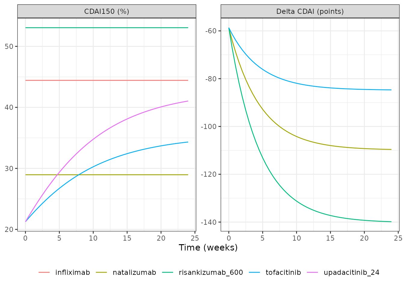
Typical-trial time course of the CDAI150 remission rate and the Delta CDAI change for selected regimens (cf. Figures 2A and 3A of Yu 2022, which plot trial-specific fits).
# The onset terms are returned by the solve: each reaches one half at the
# published ET50 and 0.9 at the ET90.
onJak <- solveArms(uis[["cdai150"]], filter(regimen, lab == "tofacitinib"), tGrid)
onAll <- solveArms(uis[["dcdai"]], filter(regimen, lab == "tofacitinib"), tGrid)
et <- c(
  et50Jak = approx(onJak$onsetJak, onJak$time, xout = 0.5)$y,
  et90Jak = approx(onJak$onsetJak, onJak$time, xout = 0.9)$y,
  et50All = approx(onAll$onsetDrug, onAll$time, xout = 0.5)$y,
  et90All = approx(onAll$onsetDrug, onAll$time, xout = 0.9)$y
)
print(round(et, 2))
#> et50Jak et90Jak et50All et90All
#>    6.30   20.93    3.16   10.47
# Results: ET50 6.3 and ET90 20.9 weeks (JAK, CDAI150); 3.2 and 10.5 weeks
# (all drugs, Delta CDAI). Linear interpolation on a 0.5-week grid.
stopifnot(
  abs(et[["et50Jak"]] - 6.3) < 0.15, abs(et[["et90Jak"]] - 20.9) < 0.3,
  abs(et[["et50All"]] - 3.2) < 0.15, abs(et[["et90All"]] - 10.5) < 0.3
)
drArms <- tibble::tribble(
  ~endpoint, ~col, ~drug,
  "cdai150", "CONMED_ADALIMUMAB_DOSE", "adalimumab",
  "cdai150", "CONMED_RISANKIZUMAB_DOSE", "risankizumab",
  "cdai150", "CONMED_PF04236921_DOSE", "PF-04236921",
  "cdai100", "CONMED_ADALIMUMAB_DOSE", "adalimumab",
  "cdai100", "CONMED_UPADACITINIB_DOSE", "upadacitinib",
  "cdai70", "CONMED_UPADACITINIB_DOSE", "upadacitinib",
  "dcdai", "CONMED_ADALIMUMAB_DOSE", "adalimumab",
  "dcrp", "CONMED_CERTOLIZUMAB_DOSE", "certolizumab pegol",
  "dcrp", "CONMED_PF04236921_DOSE", "PF-04236921",
  "dcrp", "CONMED_UPADACITINIB_DOSE", "upadacitinib",
  "dibdq", "CONMED_ADALIMUMAB_DOSE", "adalimumab",
  "dibdq", "CONMED_RISANKIZUMAB_DOSE", "risankizumab"
)
maxDose <- c(adalimumab = 160, risankizumab = 600, `PF-04236921` = 200,
             upadacitinib = 24, `certolizumab pegol` = 400)
dr <- bind_rows(lapply(seq_len(nrow(drArms)), function(i) {
  a <- drArms[i, ]
  doses <- seq(0, maxDose[[a$drug]], length.out = 25)
  arms <- tibble(lab = a$drug, col = a$col, dose = doses)
  sol <- solveArms(uis[[a$endpoint]], arms, 12)
  scale <- if (binary[[a$endpoint]]) 100 else 1
  tibble(endpoint = a$endpoint, drug = a$drug, dose = doses,
         value = scale * sol[[outNames[[a$endpoint]]]])
}))
ggplot(dr, aes(dose, value, colour = drug)) +
  geom_line() +
  facet_wrap(~endpoint, scales = "free") +
  labs(x = "Dose column value (mg)", y = "Week-12 prediction", colour = NULL) +
  theme_bw() +
  theme(legend.position = "bottom")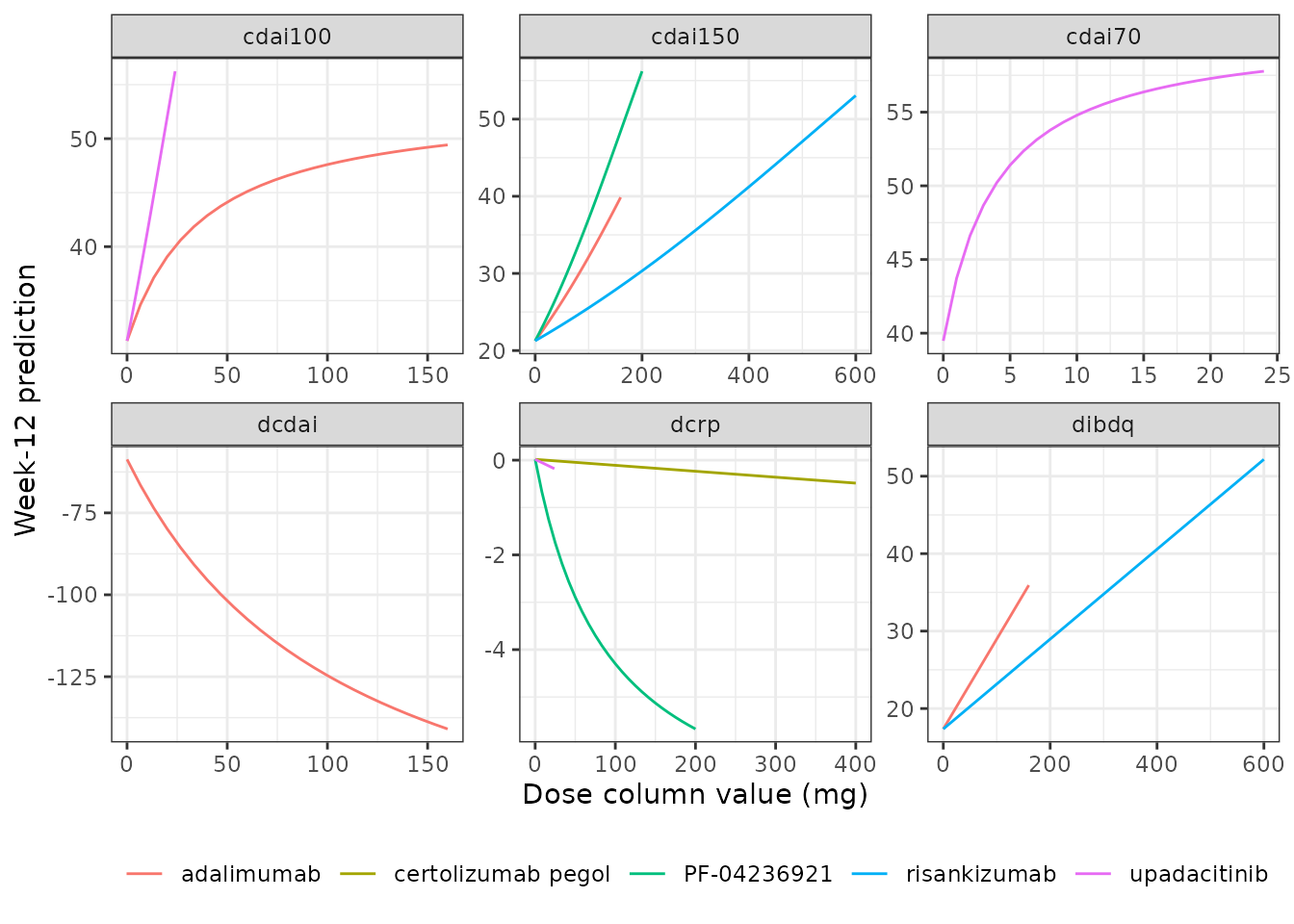
Typical-trial Week-12 dose-response of the dose-dependent drugs in each model.
Residual error at the arm level
The residual SD of an arm’s outcome shrinks with the arm size
N_ARM. It is the binomial standard error times a multiplier
for the responder rates, and addSd / sqrt(N_ARM) for the
changes from baseline. A stochastic solve of 200 replicate infliximab
arms of 100 patients at Week 12 shows the spread one arm-level
observation carries. The 200 arms are within the per-arm cap for
simulated cohorts.
rxode2::rxSetSeed(20220317)
armsRes <- regimen |> filter(lab == "infliximab")
dRes <- makeArmData(uis[["cdai150"]], armsRes[rep(1, 200), ], times = 12)
simRes <- rxode2::rxSolve(uis[["cdai150"]], dRes, returnType = "data.frame")
resSummary <- tibble(
  typical = 100 * simRes$prob_cdai150[1],
  medianSim = 100 * median(simRes$sim),
  sdSim = 100 * sd(simRes$sim),
  expectedSd = 100 * 0.837 * sqrt(simRes$prob_cdai150[1] * (1 - simRes$prob_cdai150[1]) / 100)
)
knitr::kable(resSummary, digits = 2, caption = "Simulated infliximab CDAI150 arm proportion (%), 200 arms of 100 patients.")| typical | medianSim | sdSim | expectedSd |
|---|---|---|---|
| 44.43 | 44.53 | 4.25 | 4.16 |
NCA
These models have no pharmacokinetic layer: dose enters as a covariate, there are no dose events and no concentrations, so a non-compartmental analysis does not apply. The validation above compares the models against every Week-12 prediction the paper publishes instead.
Assumptions and deviations
Placebo response
The authors estimated the placebo response non-parametrically, one
value per trial and visit, and report none of those values. For the
Week-12 simulation they fitted a separate longitudinal placebo model per
end point and report only its Week-12 value. Each model file therefore
holds the placebo term fixed at that published Week-12 value
(e0_*), constant in time. To reproduce a particular trial,
or a visit other than Week 12, replace it with that trial’s observed
placebo response (on the logit scale for the responder rates). The drug
effects are shifts relative to placebo and do not depend on this
choice.
Misprints in Supplementary Table 6 (Delta CRP)
Three Delta CRP rows are internally inconsistent in both Supplementary Table 6 and main-text Table 2. They were resolved against the midpoints of their own confidence intervals, against Figure 5B, and against a refit of the published code to the deposited dataset.
- Certolizumab pegol slope. Printed as 1.12x10^-2 with 95% CI (-1.70x10^-2, -5.47x10^-4); the estimate lies outside its interval. Encoded as -1.12x10^-3, the exact midpoint of (-1.70x10^-3, -5.47x10^-4), which reproduces the certolizumab 100, 200 and 400 mg points of Figure 5B.
- Upadacitinib slope. Printed as -0.22 (95% CI -0.43, -0.01), which gives about -5.3 at 24 mg. That would make upadacitinib the most effective CRP-lowering regimen, but the Results name PF-04236921 200 mg (-5.52) and Figure 5B plots upadacitinib 24 mg at about -0.17. Encoded as -7.3x10^-3 per mg, back-solved by the maintainers from the 24 mg point of Figure 5B relative to the natalizumab, infliximab and PF-04236921 points of the same panel, which cancels the covariate factor. The maintainers’ refit gives -8.0x10^-3. Because the value comes from Figure 5B, the upadacitinib Delta CRP points are not an independent check.
- Risankizumab effect. Printed as 4.60x10^-3 with 95% CI (5.70x10^-2, 4.78x10^-2), an interval that excludes its estimate. Encoded as -4.60x10^-3, the midpoint of (-5.70x10^-2, 4.78x10^-2), which is the reading with two dropped minus signs. The effect is negligible either way.
Conflicting baseline-CDAI exponent in the CDAI-100 model
Main-text Table 2 prints the CDAI-100 baseline-CDAI exponent as -8.77 (95% CI -14.16, -3.39); Supplementary Table 3 prints -3.21 (95% CI -7.39, 0.96). The supplement value is used. The maintainers’ refit returns -3.8 to -3.9, and the Figure 4B points are reproduced within a fraction of a percentage point with -3.21, whereas -8.77 would raise every drug effect by about 2%.
Covariate reference values
Equation 12 divides each covariate by its mean. The model code evaluates that mean over the endpoint’s analysis-dataset sheet (except in Delta CDAI, where it hard-codes 306.285). Each model uses that mean, computed from the deposited dataset after replacing missing arm values with the median arm value, as Methods ‘Available Data’ describes. That imputation reproduces the CDAI150 estimates most closely when the published code is refitted. The alternatives (the mean of the non-missing values, or a median taken over rows instead of arms) move the reference by up to about 1.5%. For the steep Delta CRP and Delta IBDQ exponents, that moves the drug effects by up to about 10% and 20%. This explains most of the common factor seen in those two panels. The paper also does not state the age of its typical simulated trial; the Table 1 overall mean, 37.20 years, is used for the Delta CRP model.
Residual error
The paper reports no residual scale. For the three responder rates,
addSd is the residual standard error of the maintainers’
refit of the published gnls() code to the deposited
dataset: 0.837 (CDAI150), 0.891 (CDAI-100) and 0.995 (CDAI-70). The same
refit returns the published fixed effects of those three models to
within about 2% (CDAI150, CDAI-70) and about 15% (CDAI-100). The
continuous models weight each arm by its own reported SD, which is
missing for most arms in the deposited dataset. The authors imputed it
with a model that is not given, so their residual scale cannot be
recovered. Those models encode a unit-scale residual with the median arm
SD of the dataset (79.4 CDAI points, 1.81 mg/dL CRP, 31.1 IBDQ points),
divided by sqrt(N_ARM). The source also fits a within-arm
autocorrelation across visits: ARMA(2) for CDAI150 and Delta CRP,
compound symmetry for CDAI-100, and AR(1) for CDAI-70, Delta CDAI and
Delta IBDQ. A per-record residual in rxode2 cannot carry it. None of
this affects the typical-value predictions.
Units of CRP
Methods ‘Data Development’ states that CRP was standardised to mg/L. However, every baseline value in Table 1 (arm means 0.67-2.98) and in the dataset is on the mg/dL scale typical of moderate-to-severe Crohn’s disease trials. The Delta CRP output and the baseline-CRP covariate are therefore labelled mg/dL. The covariate power terms are unit-free provided the column and its reference share a unit.
Dose metric
Methods ‘Data Development’ says dose regimens were normalised by
daily dose (its example: upadacitinib 12 mg twice daily as 24 mg daily).
The deposited dataset does not follow that for most drugs. Upadacitinib
3/6/12/24 mg twice daily is recorded as 3/6/12/24, and the 24 mg
once-daily arm as 12. PF-04236921 and risankizumab are the dose per
administration, and adalimumab is the week-0 induction dose.
Weight-based regimens are mg at 70 kg in every sheet except IBDQ, which
records mg/kg. The model code multiplies the dataset DOSE
directly, so each dose-response parameter is on the dataset’s scale, and
the CONMED_<drug>_DOSE columns take the dataset’s
values (see each column’s notes). Reproducing the Figure 4B
and 4C upadacitinib points with the per- administration value confirms
this reading. For the constant-effect drugs the magnitude is not
read.
Other source notes
- The supplementary table footnote gives the Emax dose-response as
Emax * dose / (ED50 * dose); the model code hasDOSE + exp(led50), which is used. - Supplementary Table 5 lists etanercept as ‘25 mg/kg biw’; the regimen is 25 mg twice weekly (Table 1 and the dataset).
- The residual-rounded risankizumab Delta IBDQ slope, 0.05 (95% CI 0.01, 0.10), has an interval midpoint of 0.055, which explains the small under-prediction of the two risankizumab points of Figure 5C.
- The caption of Figures 4 and 5 says “placebo-corrected”, but the plotted values include the placebo response (see above).
-
SCORE_CDAI,CRP,AGEandT_DIAG_CDare study-arm means, as in the source dataset, not patient values. The models describe trial arms and must not be used to simulate individual patients.