Missing dosing history in population PK (Wang 2019)
Source:vignettes/articles/Wang_2019_missing_dosing_history.Rmd
Wang_2019_missing_dosing_history.RmdModel and source
- Citation: Wang Y, Liu X. Handling Missing Dosing History in Population Pharmacokinetic Modeling: An Extension to MDM Method. CPT Pharmacometrics Syst Pharmacol. 2019;8(1):39-49. doi:10.1002/psp4.12374. PMCID PMC6363138. Structural parameter values transcribed from Table 1 (parameter set A) and cross-checked against the authors’ deposited data-generating NONMEM control stream in Code Examples S1 (supplementary file PSP4-8-39-s003 .txt, $PROB RUN# 011_1, the $SIMULATION problem), which uses exactly these values.
- Article: https://doi.org/10.1002/psp4.12374
- Open access: PMC6363138
Wang and Liu (2019) is a methodology paper, not a drug report. There is no real molecule and there are no real patients. The authors defined the population PK parameters of a hypothetical drug, simulated cohorts of 100 virtual subjects, then deleted dosing records from the simulated data sets and compared how six analysis methods recovered the parameters they had started from:
| Method | What it does |
|---|---|
| IDM | Ideal method – fits the complete data set. The reference. |
| OM | Omit method – comments out the missing dose and the observations that follow it. |
| PDM | Prescribed dose method – fills the gap with the prescribed dose (8 mg). |
| MDM |
Missing dose method (Soy 2004) – estimates an initial
amount A0 in the central compartment. |
| MDM2 |
New in this paper – MDM plus a patient-ID split
after the gap, plus a two-population mixture on A0. |
| CIM |
New in this paper – compartment
initialization: back-calculates A0 = Conc x V from the
first observation after the gap, with no extra parameter. |
Because there is no drug, these models are filed under
inst/modeldb/pharmacokinetics/ rather than
specificDrugs/, following the precedent of
Beal_2001_iv1cmt_bql and the
Schoning_2026_oral1cmt_* family, and the file stem carries
the structural descriptor oral1cmt in the slot where a drug
name would normally sit.
What is, and is not, extractable here
The data-generating model is fully specified: Table
1 gives every value, and the authors deposited the actual NONMEM
$SIMULATION control stream in Code Examples S1. That model
is packaged here, in two files matching the authors’ own split (“base
models and covariate models were separately simulated”):
nlmixr2lib::modeldb |>
  dplyr::filter(name %in% c("Wang_2019_oral1cmt_base", "Wang_2019_oral1cmt_covariate")) |>
  dplyr::select(name, parameters, dosing) |>
  dplyr::rename("Model" = name, "Parameters" = parameters,
                "Dosing compartments" = dosing) |>
knitr::kable()| Model | Parameters | Dosing compartments |
|---|---|---|
| Wang_2019_oral1cmt_base | ka,cl,vc | depot,central |
| Wang_2019_oral1cmt_covariate | ka,cl,vc,cl,vc,cl | depot,central |
The fitted arms (OM, PDM, MDM, MDM2, CIM, IDM) are
not packaged, because the paper publishes no point estimates
for them at all – only relative estimation error (Figures 2, 3) and
standardized RMSE (Tables 3, 4) summaries over 100 replicates. The
$THETA values in their deposited control streams are
deliberately offset initial estimates (CL 20 against a truth of
15, V 120 against 100, $OMEGA 0.09 against 0.04), not
results. An ini() block for those arms would have nothing
to put in it.
base <- readModelDb("Wang_2019_oral1cmt_base")()
cov  <- readModelDb("Wang_2019_oral1cmt_covariate")()
Population
The virtual cohort (Table S1, and “PK data simulation”):
- 100 subjects per data set – 50 men, 50 women.
- Weight normally distributed: men 70 (10) kg, women 60 (10) kg.
- Three doses at 0, 12 and 24 h (Table 2), oral or i.v. bolus.
- Each administered dose drawn from Uniform(5, 10) mg, although the prescribed dose is 8 mg every 12 h. This gap between prescription and reality is the whole point: it is what makes PDM biased.
- 12 samples per subject at 11.83, 12.25, 12.75, 13, 17, 23.83, 24.25, 24.75, 25, 27, 31 and 35 h, giving 1,200 observations per data set.
Source trace
Every value in both ini() blocks, with the location it
came from. The paper and the deposited control stream agree on every
one.
| Parameter | Value | Table 1 | Code Examples S1 ($PROB RUN# 011_1) |
|---|---|---|---|
lka |
log(2) |
ka = 2 (1/h) |
$THETA 2 ;[KA, 1/h] |
lcl |
log(15) |
CL = 15 L/h (set A) |
$THETA 15 ;[CL, L/h] |
lvc |
log(100) |
V = 100 L |
$THETA 100 ;[V, L] |
e_wt_cl |
0.75 |
beta1, weight influence on CL |
$THETA 0.75 ;[CLWT],
CLWT=(WT/70)**THETA(4)
|
e_wt_vc |
1 |
beta2, weight influence on V |
$THETA 1.0 ;[VWT],
VWT=(WT/70)**THETA(6)
|
e_sexf_cl |
-0.3 |
alpha, “Male: -0.3, female: 0” |
$THETA -0.3 ;[CLSEX],
TVCL=...*(1 + CLSEX*SEX)
|
etalcl |
0.04 | variance of BSV on CL (20% CV) |
$OMEGA 0.04 omega(1,1),
CL=TVCL*EXP(ETA(1))
|
etalvc |
0.04 | variance of BSV on V (20% CV) |
$OMEGA 0.04 omega(2,2),
V=TVV*EXP(ETA(2))
|
propSd |
0.1 |
sigma1^2 = 0.01 (10% CV) |
$SIGMA 0.01 ;[P] sigma(1,1) |
addSd |
1 |
sigma2^2 = 1 (ng/mL) |
$SIGMA 1 ;[A] sigma(2,2) |
F = 1 |
(no term) | “F … 1 fixed” | no F1 statement in $PK (ADVAN2
default) |
| ng/mL scaling | * 1000 |
concentrations reported in ng/mL | S2=V/1000 |
Structural verification against closed forms
This model defines variables named cl and
vc, which can make rxode2 match a system against its
analytic kernel and silently discard the explicit d/dt()
bodies. Here the ODEs are ADVAN2 TRANS2, so an analytic match
would be equivalent rather than wrong – but that must be demonstrated,
not assumed. First confirm both states survive the solve:
Now pin the solved profile to the closed form for each route. Both sides use the same parameter values, so the only difference is solver quadrature error and a tight bound is the correct gate.
D   <- 7 # mg
cl0 <- 15; vc0 <- 100; ka0 <- 2; kel0 <- cl0 / vc0
typ <- rxode2::zeroRe(base)
grid <- sort(unique(c(seq(0, 36, by = 0.25), exp(seq(log(1e-3), log(1), length.out = 30)))))

# Oral: dose into the depot
s_oral <- rxode2::rxSolve(
  typ, rxode2::et(amt = D, cmt = "depot") |> rxode2::et(grid),
  returnType = "data.frame"
)
#> ℹ omega/sigma items treated as zero: 'etalcl', 'etalvc'
cf_oral <- 1000 * D * ka0 / (vc0 * (ka0 - kel0)) *
  (exp(-kel0 * s_oral$time) - exp(-ka0 * s_oral$time))

# IV bolus: dose straight into central
s_iv <- rxode2::rxSolve(
  typ, rxode2::et(amt = D, cmt = "central") |> rxode2::et(grid),
  returnType = "data.frame"
)
#> ℹ omega/sigma items treated as zero: 'etalcl', 'etalvc'
cf_iv <- 1000 * D / vc0 * exp(-kel0 * s_iv$time)

relerr <- function(a, b) max(abs(a - b) / pmax(b, 1e-9))
c(oral = relerr(s_oral$Cc, cf_oral), iv = relerr(s_iv$Cc, cf_iv))
#>         oral           iv
#> 9.898037e-07 2.191197e-08
stopifnot(
  relerr(s_oral$Cc, cf_oral) < 1e-5,
  relerr(s_iv$Cc, cf_iv) < 1e-5,
  all(s_iv$depot == 0) # an i.v. bolus must never populate the depot
)
The covariate model reproduces its reference subject exactly
The authors’ clearance line is
TVCL = THETA(1) * CLWT * (1 + CLSEX*SEX) with
SEX = 1 for men, so
THETA(1) = 15 L/h is the clearance of a 70 kg
woman, and men clear 30% more slowly. The canonical
covariate column is SEXF (1 = female), so the effect is
applied as (1 + e_sexf_cl * (1 - SEXF)) – the construction
ratified for male-indicator sources in
Bajaj_2017_nivolumab.R and
Wada_2023_sparsentan.R. That must land on exactly 15 and
10.5 L/h:
typc <- rxode2::zeroRe(cov)
iv_ev <- function(sexf, wt) {
  e <- as.data.frame(rxode2::et(amt = D, cmt = "central") |> rxode2::et(grid))
  e$SEXF <- sexf
  e$WT <- wt
  e
}
s_w70 <- rxode2::rxSolve(typc, iv_ev(1, 70), returnType = "data.frame")
#> ℹ omega/sigma items treated as zero: 'etalcl', 'etalvc'
s_m70 <- rxode2::rxSolve(typc, iv_ev(0, 70), returnType = "data.frame")
#> ℹ omega/sigma items treated as zero: 'etalcl', 'etalvc'
s_w50 <- rxode2::rxSolve(typc, iv_ev(1, 50), returnType = "data.frame")
#> ℹ omega/sigma items treated as zero: 'etalcl', 'etalvc'

stopifnot(
  # 70 kg woman: both covariate terms are exactly 1, so CL = THETA(1) = 15
  relerr(s_w70$Cc, 1000 * D / vc0 * exp(-(15 / 100) * s_w70$time)) < 1e-5,
  # 70 kg man: CL = 15 * (1 - 0.3) = 10.5
  relerr(s_m70$Cc, 1000 * D / vc0 * exp(-(10.5 / 100) * s_m70$time)) < 1e-5,
  # mutation control: the weight term must actually be live
  max(abs(s_w50$Cc - s_w70$Cc) / s_w70$Cc) > 0.01
)
c(CL_woman70 = unique(s_w70$cl), CL_man70 = unique(s_m70$cl))
#> CL_woman70   CL_man70
#>       15.0       10.5
Replicating Figure 1: the four missing-record cases
Figure 1 illustrates the i.v. dosing situation. The underlying subject is the same in all four panels – what changes is only which dosing records the analyst can see. Solid segments are PK events with an available dosing record; dashed segments follow a missing one.
doses <- c(6, 9, 8) # mg at 0, 12, 24 h
prof <- rxode2::rxSolve(
  typ,
  rxode2::et(amt = doses, time = c(0, 12, 24), cmt = "central") |>
    rxode2::et(seq(0, 36, by = 0.05)),
  returnType = "data.frame"
)
#> ℹ omega/sigma items treated as zero: 'etalcl', 'etalvc'

cases <- list(
  "(a) Complete records"          = integer(0),
  "(b) 1st dose missing (case 1)" = 1L,
  "(c) 2nd dose missing (case 2)" = 2L,
  "(d) 3rd dose missing (case 3)" = 3L
)
fig1 <- dplyr::bind_rows(lapply(names(cases), function(nm) {
  miss <- cases[[nm]]
  # a PK event is "unobserved" from its own dose until the next dose
  win <- if (length(miss)) c(c(0, 12, 24)[miss], c(12, 24, Inf)[miss]) else c(Inf, Inf)
  dplyr::mutate(prof, panel = nm,
                observed = !(time >= win[1] & time < win[2]))
}))
dose_pts <- dplyr::bind_rows(lapply(names(cases), function(nm) {
  data.frame(panel = nm, time = c(0, 12, 24),
             recorded = !(seq_len(3) %in% cases[[nm]]))
}))

ggplot(fig1, aes(time, Cc)) +
  geom_line(aes(linetype = observed, group = interaction(panel, observed))) +
  geom_vline(data = dose_pts, aes(xintercept = time, colour = recorded),
             linewidth = 0.4) +
  facet_wrap(~panel, ncol = 2) +
  scale_linetype_manual(values = c("TRUE" = "solid", "FALSE" = "22"),
                        name = "dosing record available") +
  scale_colour_manual(values = c("TRUE" = "grey50", "FALSE" = "firebrick"),
                      name = "dose recorded") +
  labs(x = "Time (h)", y = "Concentration (ng/mL)",
       caption = "Replicates Figure 1 of Wang and Liu (2019); i.v. dosing, doses 6/9/8 mg.") +
  theme_bw() + theme(legend.position = "bottom")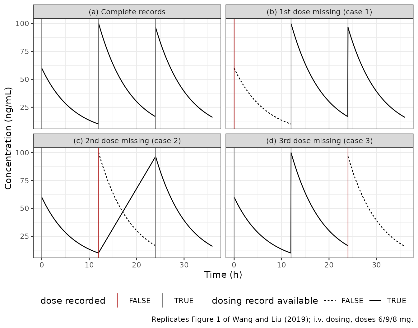
Virtual cohort and simulated trial
Reproducing the paper’s own design: 100 subjects, 50/50 sex split, weights per Table S1, three doses drawn from Uniform(5, 10) mg, and the 12 sampling times of Table 2.
rxode2::rxSetSeed(20190117)
set.seed(20190117)
n <- 100L
demog <- data.frame(
  id   = seq_len(n),
  SEXF = rep(c(0, 1), each = n / 2)
) |>
  dplyr::mutate(WT = round(stats::rnorm(n, ifelse(SEXF == 1, 60, 70), 10), 3))

samp <- c(11.83, 12.25, 12.75, 13, 17, 23.83, 24.25, 24.75, 25, 27, 31, 35)
amt_tbl <- data.frame(
  id   = rep(demog$id, each = 3),
  time = rep(c(0, 12, 24), times = n),
  amt  = round(stats::runif(3 * n, 5, 10))
)

ev <- dplyr::bind_rows(
  dplyr::transmute(amt_tbl, id, time, amt, evid = 1L, cmt = "depot"),
  data.frame(id = rep(demog$id, each = length(samp)),
             time = rep(samp, times = n),
             amt = NA_real_, evid = 0L, cmt = "central")
) |>
  dplyr::left_join(demog, by = "id") |>
  dplyr::arrange(id, time, dplyr::desc(evid))

sim <- rxode2::rxSolve(cov, ev, returnType = "data.frame")
nrow(dplyr::filter(sim, !is.na(Cc)))
#> [1] 1200
ggplot(dplyr::filter(sim, time > 0), aes(time, sim, group = id)) +
  geom_line(alpha = 0.12) +
  stat_summary(aes(group = 1), fun = median, geom = "line",
               colour = "firebrick", linewidth = 1) +
  labs(x = "Time (h)", y = "Observed concentration (ng/mL)",
       title = "Simulated oral cohort (n = 100), covariate model",
       subtitle = "Grey: individual observations with residual error. Red: median.") +
  theme_bw()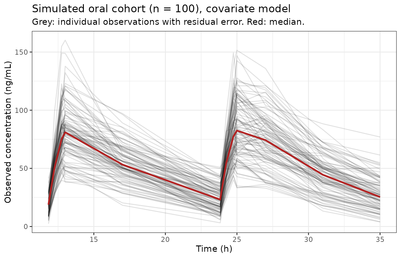
The cohort must match the demographics the paper specified:
demog |>
  dplyr::group_by(Sex = ifelse(SEXF == 1, "Female", "Male")) |>
  dplyr::summarise(n = dplyr::n(), mean_WT = round(mean(WT), 1),
                   sd_WT = round(stats::sd(WT), 1), .groups = "drop") |>
knitr::kable()| Sex | n | mean_WT | sd_WT |
|---|---|---|---|
| Female | 50 | 61.3 | 8.9 |
| Male | 50 | 69.8 | 9.1 |
PKNCA validation
The paper reports no NCA table – its results are
estimation-error summaries, not exposure metrics – so there is nothing
to compare against side by side. PKNCA is instead used for the
structural identity that must hold for any linear one-compartment model:
after a single dose, individual clearance times individual
AUCinf recovers the dose.
iv_single <- dplyr::left_join(
  dplyr::bind_rows(
    data.frame(id = demog$id, time = 0, amt = 8, evid = 1L, cmt = "central"),
    data.frame(id = rep(demog$id, each = 40), amt = NA_real_, evid = 0L,
               cmt = "central",
               time = rep(sort(unique(c(exp(seq(log(1e-3), log(72), length.out = 39)), 0))),
                          times = n))
  ),
  demog, by = "id"
) |>
  dplyr::arrange(id, time, dplyr::desc(evid))

nca_sim <- rxode2::rxSolve(cov, iv_single, returnType = "data.frame")

conc_df <- nca_sim |>
  dplyr::filter(!is.na(Cc)) |>
  dplyr::transmute(id, time, Cc, treatment = "IV 8 mg")
dose_df <- data.frame(id = demog$id, time = 0, dose = 8, treatment = "IV 8 mg")

o_conc <- PKNCA::PKNCAconc(conc_df, Cc ~ time | treatment + id,
                           concu = "ng/mL", timeu = "h")
o_dose <- PKNCA::PKNCAdose(dose_df, dose ~ time | treatment + id,
                           doseu = "mg")
res <- PKNCA::pk.nca(PKNCA::PKNCAdata(
  o_conc, o_dose,
  intervals = data.frame(start = 0, end = Inf, aucinf.obs = TRUE, half.life = TRUE)
))

nca <- as.data.frame(res) |>
  dplyr::select(id, PPTESTCD, PPORRES) |>
  tidyr::pivot_wider(names_from = PPTESTCD, values_from = PPORRES) |>
  dplyr::mutate(id = as.integer(as.character(id)))

indiv <- nca_sim |>
  dplyr::group_by(id) |>
  dplyr::summarise(cl = dplyr::first(cl), vc = dplyr::first(vc), .groups = "drop")

chk <- dplyr::left_join(nca, indiv, by = "id") |>
  dplyr::mutate(
    # Cc is ng/mL = ug/L, so cl (L/h) * AUC (ug*h/L) is ug; the dose is 8 mg.
    dose_recovery = cl * aucinf.obs / (8 * 1000),
    hl_ratio      = half.life / (log(2) * vc / cl)
  )
chk |>
  dplyr::summarise(
    `Dose recovery (cl x AUCinf / dose)` = median(dose_recovery),
    `Half-life vs ln(2)*vc/cl`           = median(hl_ratio)
  ) |>
  tidyr::pivot_longer(dplyr::everything(), names_to = "Identity",
                      values_to = "Median ratio") |>
  dplyr::mutate(`Median ratio` = round(`Median ratio`, 5)) |>
knitr::kable()| Identity | Median ratio |
|---|---|
| Dose recovery (cl x AUCinf / dose) | 1 |
| Half-life vs ln(2)*vc/cl | 1 |
Both identities are asserted on the centre and on a robust quantile, never on the cohort extreme – the extreme of a random cohort is not reproducible across rxode2 builds, whereas these medians are.
Why the missing-dose methods are needed
Two of the paper’s claims are arithmetic, and can be checked directly against this model rather than restated as prose.
PDM is biased because the prescription is not the dose. The prescribed dose is 8 mg; the administered doses are Uniform(5, 10). Filling a gap with 8 mg therefore misstates the true amount by a predictable amount:
pdm_err <- (8 - amt_tbl$amt) / amt_tbl$amt
c(`median absolute dose error` = median(abs(pdm_err)),
  `max absolute dose error`    = max(abs(pdm_err)))
#> median absolute dose error    max absolute dose error
#>                  0.1428571                  0.6000000
stopifnot(median(abs(pdm_err)) > 0.05)
CIM’s identity is exact. The compartment
initialization method sets A0(t) = Conc(t) x V, so
re-initializing the central compartment from an observed concentration
must reproduce that concentration exactly. Solving a fresh profile whose
initial central amount is back-calculated from a sampled concentration
recovers the sampled value:
# take a 70 kg woman, sample her true concentration at 11.83 h, then
# re-initialize a fresh solve from A0 = Conc * V and confirm it lands there.
probe <- rxode2::rxSolve(typc, iv_ev(1, 70), returnType = "data.frame")
#> ℹ omega/sigma items treated as zero: 'etalcl', 'etalvc'
conc_t <- approx(probe$time, probe$Cc, xout = 11.83)$y
V_i    <- unique(probe$vc)
A0     <- conc_t * V_i / 1000 # ng/mL -> mg/L, times L, gives mg

reinit <- as.data.frame(
  rxode2::et(amt = A0, cmt = "central") |> rxode2::et(c(0, 1e-6))
)
reinit$SEXF <- 1
reinit$WT <- 70
back <- rxode2::rxSolve(typc, reinit, returnType = "data.frame")
#> ℹ omega/sigma items treated as zero: 'etalcl', 'etalvc'

c(sampled = conc_t, reinitialized = back$Cc[1])
#>       sampled reinitialized
#>      11.87158      11.87158
stopifnot(abs(back$Cc[1] - conc_t) / conc_t < 1e-6)
Assumptions and deviations
Parameter set A is encoded. Table 1 lists five sets A-E differing only in clearance (15, 20, 25, 30, 35 L/h). Set A is used because it is the set the authors’ own deposited
$SIMULATIONcontrol stream actually runs ($THETA 15 ;[CL, L/h]). Changelcltolog(20)…log(35)for B-E.The weight reference is 70 kg, not the dataset median. The paper’s printed equation normalizes a continuous covariate by “the median value of the continuous covariate in the dataset”, which for a balanced cohort drawn at 70 (10) kg for men and 60 (10) kg for women is about 65 kg. The authors’ deposited control stream instead hardcodes
CLWT=(WT/70)**THETA(4)andVWT=(WT/70)**THETA(6). The executed code governs, so 70 kg is used here.Sex reference category is inverted relative to the source. The source column
SEXis a male indicator (SEX=1 IF MALE, 0 IF FEMALE), so the canonicalSEXF = 1 - SEX. The published coefficient -0.3 is preserved verbatim and applied to(1 - SEXF); consequentlylcl = log(15)is the clearance of a 70 kg woman, and men are 30% lower. Verified numerically above.Table 1’s two omega row labels are transposed. The row labelled
omega2 - Vis described as “Variance of BSV on CL” and the row labelledomega2 - CLas “Variance of BSV on V”. Both values are 0.04, so the transposition has no numerical consequence; the control stream (CL=TVCL*EXP(ETA(1)),$OMEGA 0.04 omega(1,1)) settles the mapping.The deposited data example is not from parameter set A. Data Examples S1 gives one subject (WT 64.395 kg, male, doses 6/9/8 mg) with concentrations. Its troughs decay far faster than set A allows: the observed 23.83 h trough is 2.51 ng/mL against 34.4 predicted for set A, and a least-squares fit at fixed V = 100 and ka = 2 returns CL ~ 46 L/h – above every published set, and reachable from set E (35 L/h) with a ~1.4 SD individual eta but from set A only with a ~5.6 SD one. The deposited control stream and the deposited data file therefore come from different runs. This does not affect the encoded values, which are doubly sourced from Table 1 and
$THETA, but the deposited data cannot be used as a validation target and is not used as one.Fitted-arm models are deliberately absent, as explained above: the paper publishes relative errors, not estimates.
Specimen is unverified. The paper says only that “blood samples were collected during visits and later analyzed for drug concentrations (ng/mL)”; it never states plasma, serum or whole blood, so
compartmentData$central$verifiedisFALSE.The 8 mg nominal dose and the Uniform(5, 10) actual dose are both real features of the design, not a transcription conflict – the divergence between them is the mechanism the paper is studying.