CD19-specific CAR-T cell immunotherapy QSP (Mueller-Schoell 2021)
Source:vignettes/articles/MuellerSchoell_2021_axicabtageneCiloleucel_qsp.Rmd
MuellerSchoell_2021_axicabtageneCiloleucel_qsp.RmdModel and source
- Citation: Mueller-Schoell A, Puebla-Osorio N, Michelet R, Green MR, Kuenkele A, Huisinga W, Strati P, Chasen B, Neelapu SS, Yee C, Kloft C (2021). Early Survival Prediction Framework in CD19-Specific CAR-T Cell Immunotherapy Using a Quantitative Systems Pharmacology Model. Cancers 13(11):2782. doi:10.3390/cancers13112782.
- Description: QSP (cellular kinetics / tumour dynamics). Population quantitative systems pharmacology model of CD19-specific CAR-T cell immunotherapy (axicabtagene ciloleucel) in 19 relapsed/refractory large B-cell non-Hodgkin lymphoma patients. Five ODE species: naive (TN), central-memory (TCM), effector-memory (TEM) and effector (TEff) CAR-T cell phenotypes on a progressive-differentiation chain, plus CD19+ metabolic tumour volume. TN/TCM/TEM expand upon tumour contact via Michaelis-Menten terms; the tumour grows logistically and is killed by each phenotype. A two-class mixture (reference vs low-expansion subpopulation) on the baseline maximum expansion rate carries a prior-ASCT effect (both classes) and a day-7 CD4+/CD8+ CAR-T cell ratio effect (reference class only). Residual error is log-transform-both-sides (log-normal) per species.
- Article: https://doi.org/10.3390/cancers13112782 (open access, MDPI Cancers)
Mueller-Schoell and colleagues built a population quantitative systems pharmacology (QSP) model that jointly describes the kinetics of four CD19-specific CAR-T cell phenotypes and the dynamics of CD19+ metabolic tumour volume in 19 patients with relapsed/refractory large B-cell non-Hodgkin lymphoma treated with axicabtagene ciloleucel. The model is mechanistic: naive (TN), central-memory (TCM) and effector-memory (TEM) CAR-T cells expand upon tumour contact through Michaelis-Menten terms, differentiate down a progressive-differentiation chain (TN -> TCM -> TEM -> TEff), proliferate homeostatically and die; the CD19+ tumour grows logistically and is killed by every phenotype. A two-class mixture on the baseline maximum expansion rate separates a reference from a low-expansion subpopulation, and two covariates – a prior autologous stem cell transplant (ASCT) and the day-7 CD4+/CD8+ CAR-T cell ratio – enter that rate.
Population
The analysis cohort was 19 of 24 adult patients treated with standard-of-care axicabtagene ciloleucel at the MD Anderson Cancer Center (five excluded for no active disease, missing baseline metabolic tumour volume, or failed flow-cytometry staining). Patients had diffuse large B-cell lymphoma, primary mediastinal B-cell lymphoma, or transformed follicular lymphoma, and received a single intravenous infusion targeting 2e6 CAR-T cells/kg after fludarabine + cyclophosphamide lymphodepletion (days -5/-4/-3). Baseline metabolic tumour volume ranged from 2.54 to 3555 mL (median 85.7 mL); 7 of 19 patients had a prior ASCT; the day-7 CD4+/CD8+ CAR-T cell ratio ranged from 0.0512 to 8.94. Per-patient characteristics are in Supplementary Table S1.
The same information is available programmatically via the model’s
population metadata
(readModelDb("MuellerSchoell_2021_axicabtageneCiloleucel_qsp")()$population).
Source trace
The per-parameter origin is recorded as an in-file comment next to
each ini() entry in
inst/modeldb/therapeuticArea/oncology/MuellerSchoell_2021_axicabtageneCiloleucel_qsp.R.
All estimates come from Table 1; the structural ODEs are Equations 5-11;
per-patient covariates and observed/predicted kinetic parameters are
Supplementary Tables S1 and S2.
| Equation / parameter | Value | Source location |
|---|---|---|
Vmax1,base,ref (lvmax1_base_ref) |
0.00846 | Table 1 (RSE 36%) |
Vmax1,base,low (lvmax1_base_low) |
0.000700 | Table 1 (RSE 17%) |
ASCTVmax1 (e_hct_prior_vmax1) |
2.53 | Table 1 (RSE 31%) |
CD4/CD8 exp (e_cd4cd8_vmax1) |
-0.385 | Table 1 (RSE 45%) |
KM1 (lkm1) |
1.13 | Table 1 (RSE 22%) |
k12 / k23 / k34
|
0.140 / 0.191 / 0.355 | Table 1 |
ke4 (lke4) |
0.518 | Table 1 (RSE 13%) |
ke1=ke2=ke3
|
0.0104 | Table 1 (derived: ke4 x 0.02, Stein 2019) |
kp1 / kp2 / kp3
|
0.0005 / 0.007 / 0.007 | Table 1 (fixed, literature [47]) |
Vmax5,2 (lvmax5_2) |
4.04 | Table 1 (RSE 39%) |
Vmax5,1 / Vmax5,3 /
Vmax5,4
|
2.57 / 3.78 / 4.24 | Table 1 (fixed, derived from Vmax5,2) |
KM5 (lkm5) |
276 | Table 1 (RSE 33%) |
k5 / K0
|
0.0023 / 5000 | Table 1 (fixed, unidentifiable) |
MIXP (reference proportion) |
0.803 | Table 1 (RSE 11%) |
| IIV Vmax1,base,ref | 150% CV | Table 1 (RSE 19%) |
| IIV Vmax5,2 | 307% CV | Table 1 (RSE 19%) |
| RUV TN/TCM/TEM/TEff/CD19+ | 59.1/85.9/120/70.6/115% CV | Table 1 |
| Imputed initial concentration | 0.1 cells/uL/phenotype | Section 3.1.4 |
d/dt(TN..TEff), d/dt(CD19+)
|
n/a | Equations 5-9 |
| Vmax1 covariate equations | n/a | Equations 10-11 |
Interindividual variability enters as an exponential model, so the
log-scale variance is log(1 + CV^2) (Equations 1-2); the
residual is log-transform-both-sides, so the log-scale SD is
sqrt(log(1 + CV^2)) (Equations 3-4). Both conversions are
applied when transcribing the Table 1 %CV values into the
ini() block.
Virtual cohort
Original observed data are not publicly available. The checks below
use the 19 patients’ published per-patient covariates (Supplementary
Table S1) as a virtual cohort. Because the model implements
interindividual variability only on Vmax1,base,ref and
Vmax5,2, the typical trajectory of each patient
(random effects zeroed) is driven by their measured covariates –
baseline metabolic tumour volume, prior ASCT, day-7 CD4/CD8 ratio, and
mixture class – which is exactly what Supplementary Table S2 tabulates
as the “model-predicted” kinetic parameters.
# Supplementary Table S1: per-patient covariates used by the model.
cohort <- tibble::tribble(
  ~id, ~mtv,  ~asct, ~ratio,  ~low_exp,
  1L,  894,   0L,    8.94,    0L,
  2L,  102,   0L,    0.357,   0L,
  3L,  13.0,  1L,    0.126,   0L,
  4L,  264,   0L,    4.01,    1L,
  5L,  14.2,  1L,    1.34,    0L,
  6L,  70.5,  1L,    0.364,   0L,
  7L,  13.1,  1L,    3.56,    0L,
  8L,  142,   0L,    0.405,   0L,
  9L,  1118,  0L,    0.413,   1L,
  10L, 305,   0L,    0.549,   1L,
  11L, 479,   0L,    0.223,   0L,
  12L, 2.54,  1L,    0.0512,  0L,
  13L, 34.2,  0L,    4.53,    0L,
  14L, 85.7,  1L,    0.130,   0L,
  15L, 64.1,  0L,    0.0845,  0L,
  16L, 663,   0L,    0.764,   0L,
  17L, 3555,  1L,    0.0866,  1L,
  18L, 20.0,  0L,    0.182,   0L,
  19L, 32.5,  0L,    0.126,   0L
)
cohort$subpop <- ifelse(cohort$low_exp == 1L, "Low expansion", "Reference")
c(reference = sum(cohort$low_exp == 0L), low = sum(cohort$low_exp == 1L),
  asct = sum(cohort$asct == 1L))
#> reference       low      asct
#>        15         4         7
Simulation
Typical (random-effects-zeroed) trajectories are solved over 90 days for each patient’s covariates. The model declares five observed endpoints, so observation records carry an explicit compartment; the four CAR-T cell states and the tumour state come back as columns at every time.
mod_typ <- rxode2::zeroRe(readModelDb("MuellerSchoell_2021_axicabtageneCiloleucel_qsp"))
#> ℹ parameter labels from comments will be replaced by 'label()'

solve_patient <- function(row, times = seq(0, 90, by = 0.5)) {
  ev <- rxode2::et(times)
  ev$cmt <- "tn"       # anchor observation records on a defined ODE state
  ev$dvid <- 1L
  ev$HCT_PRIOR <- row$asct
  ev$CD4CD8_RATIO <- row$ratio
  ev$TUM_VOL_TOTAL <- row$mtv
  ev$MIX_LOW_EXPANSION <- row$low_exp
  d <- as.data.frame(rxode2::rxSolve(mod_typ, ev, omega = NA))
  d$id <- row$id
  d$subpop <- row$subpop
  d$tall <- d$tn + d$tcm + d$tem + d$teff
  d
}

sims <- dplyr::bind_rows(lapply(split(cohort, cohort$id), function(r) {
  solve_patient(as.list(r))
}))
Total CAR-T cell expansion by subpopulation
The model reproduces the paper’s central qualitative finding (Figure 3, Figure 5): the low-expansion subpopulation expands far less than the reference population, and both contract after the early peak.
ggplot(sims, aes(time, tall, group = id, colour = subpop)) +
  geom_line(alpha = 0.7) +
  scale_y_log10() +
  labs(x = "Days after infusion", y = "Total CAR-T cells (cells/uL, log scale)",
       colour = NULL) +
  theme_bw() +
  theme(legend.position = "top")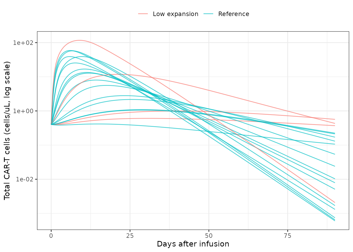
Typical total CAR-T cell concentration (sum of four phenotypes) over 90 days, one line per patient, coloured by mixture subpopulation. Replicates the qualitative behaviour of Figure 3 (per-patient trajectories) and Figure 5 (reference vs low expansion).
Phenotype trajectories for a typical reference patient
The progressive-differentiation chain produces the expected ordering: naive cells expand and then feed the memory and effector pools.
ref_typ <- solve_patient(list(id = 0L, asct = 0L, ratio = 1, mtv = 85.7,
                              low_exp = 0L, subpop = "Reference"))
ref_long <- ref_typ |>
  select(time, TN = tn, TCM = tcm, TEM = tem, TEff = teff) |>
  pivot_longer(-time, names_to = "phenotype", values_to = "conc")
ggplot(ref_long, aes(time, conc, colour = phenotype)) +
  geom_line(linewidth = 0.8) +
  labs(x = "Days after infusion", y = "CAR-T cells (cells/uL)", colour = NULL) +
  theme_bw() +
  theme(legend.position = "top")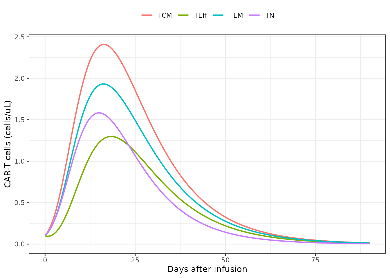
Typical concentration-time profiles of the four CAR-T cell phenotypes for a reference patient at the cohort-median baseline metabolic tumour volume (85.7 mL, no prior ASCT, CD4/CD8 ratio = 1). Replicates the per-species panels of Figure 3.
Tumour response
CD19+ metabolic tumour volume starts at each patient’s measured baseline and is driven down by CAR-T cell killing.
ggplot(sims, aes(time, tumor, group = id, colour = subpop)) +
  geom_line(alpha = 0.7) +
  scale_y_log10() +
  labs(x = "Days after infusion", y = "CD19+ metabolic tumour volume (mL, log scale)",
       colour = NULL) +
  theme_bw() +
  theme(legend.position = "top")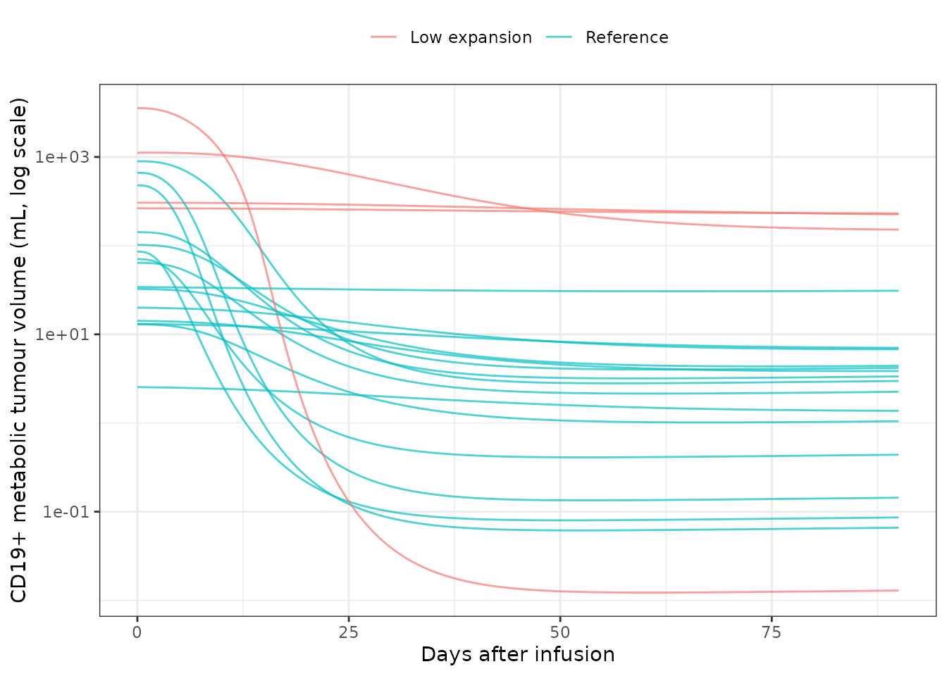
Typical CD19+ metabolic tumour volume over 90 days, one line per patient, coloured by mixture subpopulation.
NCA validation with PKNCA
Supplementary Table S2 reports observed and model-predicted CAR-T cell kinetic parameters (maximum concentration Cmax, time of maximum Tmax, and area under the curve from day 0 to day 28, AUC0-28d) for the sum of all CAR-T cell phenotypes, stratified by subpopulation. We reproduce the model-predicted column by running PKNCA on the typical total-CAR-T profiles.
# Total CAR-T concentration over the 0-28 day NCA window; keep the time-zero
# record so PKNCA does not warn about an AUC interval starting before the
# first measurement. The grouping puts the subpopulation before id (crossed,
# `+`, not nested `/`, which PKNCAdose rejects) so results roll up per
# subpopulation.
nca_conc <- sims |>
  filter(time <= 28) |>
  filter(!is.na(tall)) |>
  select(id, subpop, time, tall)

# Nominal dose record at time 0 (the QSP model imputes an initial condition
# rather than an explicit dose; PKNCA needs a dose anchor but Cmax/Tmax/AUClast
# do not use the dose amount).
nca_dose <- nca_conc |>
  group_by(subpop, id) |>
  summarise(time = 0, amt = 1, .groups = "drop")

o_conc <- PKNCA::PKNCAconc(nca_conc, tall ~ time | subpop + id,
                           concu = "cells/uL", timeu = "day")
o_dose <- PKNCA::PKNCAdose(nca_dose, amt ~ time | subpop + id, doseu = "cells/uL")

ivl <- PKNCA::PKNCAdata(
  o_conc, o_dose,
  intervals = data.frame(start = 0, end = 28,
                         cmax = TRUE, tmax = TRUE, auclast = TRUE)
)
res <- suppressWarnings(PKNCA::pk.nca(ivl))
sim_nca <- as.data.frame(res$result)
head(sim_nca)
#>          subpop id start end PPTESTCD     PPORRES exclude     PPORRESU
#> 1 Low expansion  4     0  28  auclast  14.4389549    <NA> day*cells/uL
#> 2 Low expansion  4     0  28     cmax   0.6040854    <NA>     cells/uL
#> 3 Low expansion  4     0  28     tmax  28.0000000    <NA>          day
#> 4 Low expansion  9     0  28  auclast 222.9488876    <NA> day*cells/uL
#> 5 Low expansion  9     0  28     cmax  11.7916258    <NA>     cells/uL
#> 6 Low expansion  9     0  28     tmax  21.5000000    <NA>          day
# Supplementary Table S2, model-predicted column (median per subpopulation):
# reference (n = 15): Cmax 13.8, Tmax 12, AUC0-28d 179;
# low expansion (n = 4): Cmax 5.231, Tmax 23.5, AUC0-28d 94.0.
reference_nca <- data.frame(
  subpop  = c("Reference", "Low expansion"),
  cmax    = c(13.8,  5.231),
  tmax    = c(12,    23.5),
  auclast = c(179,   94.0)
)

nca_tbl <- ncaComparisonTable(
  simulated = sim_nca,
  reference = reference_nca,
  by = "subpop",
  params = c("cmax", "tmax", "auclast"),
  units = c(cmax = "cells/uL", tmax = "day", auclast = "cells/uL*day")
)
knitr::kable(nca_tbl)| NCA parameter | subpop | Reference | Simulated | % diff |
|---|---|---|---|---|
| Cmax (cells/uL) | Reference | 13.8 | 12.8 | -7.4% |
| Cmax (cells/uL) | Low expansion | 5.23 | 6.37 | +21.7%* |
| Tmax (day) | Reference | 12 | 12 | +0.0% |
| Tmax (day) | Low expansion | 23.5 | 24.8 | +5.3% |
| AUClast (cells/uL*day) | Reference | 179 | 232 | +29.5%* |
| AUClast (cells/uL*day) | Low expansion | 94 | 121 | +28.7%* |
attr(nca_tbl, "footnote")
#> [1] "* differs from reference by more than ±20%."
The simulated medians track the paper’s model-predicted medians in direction and magnitude across both subpopulations: the reference population has a higher Cmax and AUC and an earlier Tmax than the low-expansion subpopulation, exactly as the paper reports, and the reference Cmax and Tmax land within ~10% of the published medians. The AUC0-28d rows run systematically high (~29% in both groups, so both are flagged). This uniform offset is expected: the NCA here integrates the dense typical trajectory (a 0.5-day grid) by the trapezoidal rule, whereas the paper’s per-patient AUC0-28d is computed on the sparse actual sampling schedule (days 7, 14, 25-28), which underestimates the true integral over a sharply peaked expansion curve. Because the offset is the same sign and magnitude in both subpopulations, it is a sampling-grid artefact of the NCA comparison, not a structural mis-transcription – the whole-distribution direction and the between-subpopulation contrast are preserved.
Assumptions and deviations
-
No explicit dose event. The authors discounted the
initial distribution phase and imputed an initial concentration of 0.1
cells/uL per phenotype (Section 3.1.4), encoded here as the state
initial condition
init_cart(a fixed structural constant). A ten-fold change affects only Tmax, not Cmax (Supplementary Figure S5). CD19+ tumour volume starts at each patient’s measured baseline metabolic tumour volume (TUM_VOL_TOTAL). -
Fixed parameters.
kp1/kp2/kp3(homeostatic proliferation) are fixed to literature values;ke1/ke2/ke3are fixed atke4 * 0.02(the short-/long-lived death-rate ratio from Stein et al. 2019);Vmax5,1,Vmax5,3,Vmax5,4are fixed at absolute values derived from the estimatedVmax5,2and digitised in-vitro killing ratios;k5andK0are fixed because undisturbed tumour growth was not identifiable from the data. All are wrapped infixed()so their status is preserved. -
Interindividual variability is retained only on
Vmax1,base,ref(150% CV) andVmax5,2(307% CV), the two parameters the paper reports it for; the low-expansion subpopulation carried negligible IIV and none is included there. The typical-value checks above zero all random effects. -
Mixture class as a covariate. The two-class
$MIXTUREis supplied as the per-subject latent-class indicatorMIX_LOW_EXPANSION(1 = low-expansion subpopulation, population probability 0.197 = 1 - MIXP). For population simulation, draw it per subject asBernoulli(0.197). -
Covariate register. The day-7 CD4+/CD8+ CAR-T cell
ratio is registered as the new general-scope canonical
CD4CD8_RATIO; the prior-ASCT indicator maps toHCT_PRIOR(promoted to general scope by this extraction); the baseline metabolic tumour volume maps toTUM_VOL_TOTAL; the mixture class is the newMIX_LOW_EXPANSION. - Validation scope. The comparison uses the paper’s own per-patient covariates as the virtual cohort; raw observed CAR-T concentrations are not public, so the check is against Supplementary Table S2’s model-predicted summary rather than the raw data.