Non-Hodgkin lymphoma progression-free survival (Li 2017)
Source:vignettes/articles/Li_2017_nhl_pfs.Rmd
Li_2017_nhl_pfs.RmdModel and source
mod <- rxode2::rxode2(readModelDb("Li_2017_nhl_pfs_mbma"))
#> ℹ parameter labels from comments will be replaced by 'label()'
Citation: Li M, Dave N, Salem AH, Freise KJ. Model-based meta-analysis of progression-free survival in non-Hodgkin lymphoma patients. Medicine (Baltimore). 2017;96(35):e7988. doi:10.1097/MD.0000000000007988. The model equation, the covariate-model narrative and the final parameter estimates are in the Supplemental Content (Model Description; Table S1), http://links.lww.com/MD/B853; the main text carries no parameter table.
Supplemental Content (Model Description, Figure S1, Table S1): http://links.lww.com/MD/B853, also available as
medi-96-e7988-s001.docxfrom https://europepmc.org/article/PMC/PMC5585532Description: MBMA. Model-based meta-analysis of PROGRESSION-FREE SURVIVAL (PFS) in non-Hodgkin lymphoma (NHL), fitted to study-arm-level summary PFS Kaplan-Meier curves digitised from 112 published clinical trials (155 cohorts, 11,824 patients, 3,098 observations, reported 1993-2015). PFS time follows a two-parameter Weibull distribution S(t) = exp(-(t / lambda)^k) with scale lambda = 110 months and shape (Weibull slope) k = 0.79 in the reference cohort, so the median PFS time is lambda * log(2)^(1/k) = 69.1 months. The reference cohort is rituximab as the only treatment, 100% mantle cell lymphoma (MCL) and 100% treatment-naive. Three covariate blocks act log-linearly on lambda and none was retained on k: cohort regimen (rituximab, CHOP/CHOP-like, bendamustine, other non-chemotherapy drugs; bortezomib and other chemotherapy were eliminated), the cohort’s NHL-histology mix (follicular lymphoma, DLBCL, other NHL against an MCL reference), and the cohort’s fraction of treatment-experienced patients. Because the median PFS time is directly proportional to lambda, each coefficient exponentiates to a median-PFS-time ratio: bendamustine 4.0-fold, rituximab 3.1-fold, CHOP/CHOP-like 2.3-fold, other drugs 2.3-fold, follicular lymphoma 1.6-fold, DLBCL 0.24-fold and an all-treatment-experienced cohort 0.16-fold. Variability is MBMA-specific and between-STUDY only: inter-study variance 1.4 on log-lambda and 0.17 on log-k. There is no ODE, no dosing and no PK layer; time is in months and the model outputs the progression-free probability sur, the cumulative hazard cumhaz and the median PFS time tmed. Suitable simulation scope is study-arm PFS curves, median PFS times and between-arm hazard ratios, NOT individual-patient event times. Parameter values are Supplemental Content Table S1 (Final Model column); the Weibull form is Supplemental Content Model Description equation 1, whose published rendering carries a typesetting error corrected here (see the vignette Errata).
The main text of Li 2017 contains no parameter table and no model equation. Both live in the Supplemental Content, which the Methods and Results sections point to. Everything transcribed below comes from that document; no value is taken from the abstract or from a figure.
Population
The model was fitted to study-arm-level summary progression-free survival (PFS) Kaplan-Meier curves digitised from published non-Hodgkin lymphoma (NHL) trials. Of 513 NHL trials screened from PubMed, FDA reviews, clinicaltrials.gov and the ASCO / ASH proceedings for 1993-2015, 179 met the inclusion criteria, 17 were removed as duplicates, and 50 of the remaining 162 were dropped for not reporting a PFS Kaplan-Meier curve. The analysis dataset is therefore 112 studies, 155 cohorts (arms or strata), 11,824 patients and 3,098 observations, of which 22 studies were randomised (Li 2017 Figure 1 and Results).
Cohort-level characteristics (Li 2017 Table 1): median age 63 years across cohorts (range of cohort medians 47-83; not reported in 8 cohorts, 5.1%); median 59% male patients (range 29-91%; not reported in 14 cohorts, 9%). Histology strata: DLBCL 49 cohorts (31.6%), follicular lymphoma 44 (28.4%), mantle cell lymphoma 33 (21.3%), mixed 25 (16.1%), other 4 (2.5%). Treatment coverage, which overlaps because a cohort can appear in several levels: rituximab 98 cohorts (63.2%), other non-chemotherapy drugs 60 (38.7%), CHOP/CHOP-like 41 (26.4%), other chemotherapy 36 (23.2%), bortezomib 22 (14.2%), bendamustine 11 (7%).
No dose information was modelled. Li 2017 Discussion states that treatment duration, drug potency and dose “were not considered in the model development, as there were not sufficient details available for many of the trials”, so every treatment covariate is a presence/absence indicator. There is likewise no PK layer and no exposure metric.
The same information is available programmatically via the model’s
population metadata
(readModelDb("Li_2017_nhl_pfs_mbma")()$population).
Source trace
Every ini() entry in
inst/modeldb/therapeuticArea/oncology/Li_2017_nhl_pfs_mbma.R
carries an in-file comment naming its source row. The table collects
them.
| Equation / parameter | Value | Source location |
|---|---|---|
Weibull survivor PFS(t) = exp(-(t/lambda)^k)
|
n/a | Supplemental Content, Model Description, equation (1) – as printed the equation is defective; see Errata |
Log-linear (“exponential”) covariate model on
lambda
|
n/a | Supplemental Content, Model Description (“Exponential model centered by median covariate value”; reference population = rituximab only / MCL / 100% treatment-naive) |
Residual = scalar x SE of ln(-ln(PFS(t)))
|
n/a | Supplemental Content, Model Description (citing Arends 2008) |
lk (shape k) |
0.79 | Table S1, Final Model, row k (RSE 4.3%, 95% CI 0.72, 0.85) |
llambda (scale lambda, months) |
110 | Table S1, Final Model, row lambda (RSE 26.5%, 95% CI 52.8, 167.2) |
e_norituximab_llambda |
-1.13 | Table S1, Final Model, row “No rituximab on lambda” (RSE 9.4%, 95% CI -1.34, -0.92) |
e_chop_llambda |
0.819 | Table S1, Final Model, row “CHOP/CHOP-like on lambda” (RSE 26.7%, 95% CI 0.39, 1.25) |
e_nonchemoother_llambda |
0.813 | Table S1, Final Model, row “Other drugs on lambda” (RSE 8%, 95% CI 0.69, 0.94) |
e_bendamustine_llambda |
1.39 | Table S1, Final Model, row “Bendamustine on lambda” (RSE 15.7%, 95% CI 0.96, 1.82) |
e_fl_llambda |
0.46 | Table S1, Final Model, row “Follicular lymphoma on lambda” (RSE 25%, 95% CI 0.23, 0.68) |
e_dlbcl_llambda |
-1.41 | Table S1, Final Model, row “DLBCL on lambda” (RSE 8.5%, 95% CI -1.64, -1.18) |
e_othernhl_llambda |
-0.17 | Table S1, Final Model, row “Other lymphomas on lambda” (RSE 113%, 95% CI -0.54, 0.21) |
e_experienced_llambda |
-1.85 | Table S1, Final Model, row “% experienced patients on lambda” (RSE 12.8%, 95% CI -2.32, -1.39) |
eta_study_lk (variance) |
0.17 | Table S1, Final Model, row omega^2_k (RSE 13.4%, shrinkage 5%) |
eta_study_llambda (variance) |
1.4 | Table S1, Final Model, row omega^2_lambda (RSE 14.5%, shrinkage 2.3%) |
expSd (= sqrt of the tabulated variance) |
1.0954451 | Table S1, Final Model, row sigma^2 = 1.2 (RSE 14.0%, shrinkage 3.4%) |
| Time unit = month | n/a | Li 2017 Figure 2 x-axis, “Time(month)” |
Cohort characteristics in population
|
n/a | Li 2017 Table 1 and Results |
Internal-validation percentages in population
|
n/a | Li 2017 Methods and Results |
Every tabulated value is checked against the loaded model below, so a transcription slip fails the render rather than shipping.
theta <- mod$theta
published <- c(
  lk                      = log(0.79),
  llambda                 = log(110),
  e_norituximab_llambda   = -1.13,
  e_chop_llambda          = 0.819,
  e_nonchemoother_llambda = 0.813,
  e_bendamustine_llambda  = 1.39,
  e_fl_llambda            = 0.46,
  e_dlbcl_llambda         = -1.41,
  e_othernhl_llambda      = -0.17,
  e_experienced_llambda   = -1.85,
  expSd                   = sqrt(1.2)
)
stopifnot(
  setequal(names(theta), names(published)),
  isTRUE(all.equal(theta[names(published)], published, tolerance = 1e-7))
)

# Table S1 reports omega^2 and sigma^2 as VARIANCES, so the diagonal of
# omega is used as tabulated and expSd is the square root of sigma^2.
stopifnot(
  isTRUE(all.equal(
    diag(mod$omega)[c("eta_study_lk", "eta_study_llambda")],
    c(eta_study_lk = 0.17, eta_study_llambda = 1.4),
    tolerance = 1e-12
  )),
  abs(theta[["expSd"]]^2 - 1.2) < 1e-7
)
Structural model
PFS time follows a two-parameter Weibull distribution. In the scale /
shape parameterisation the Supplemental Content defines
(lambda the scale, k the shape, “also known as
the Weibull slope”):
The second form is the Weibull probability-plot linearisation, in
which k is literally the slope against ln t –
which is what the phrase “Weibull slope” names, and which is the scale
the residual error was entered on. The model exposes the cumulative
hazard cumhaz
,
the progression-free probability sur
,
and the median PFS time
which is directly proportional to
lambda. That proportionality is why every
covariate coefficient in Table S1 exponentiates to a median-PFS-time
ratio, and it is what makes the Li 2017 Figure 3 panels an exact
arithmetic check on the transcription rather than a visual one.
Three covariate blocks act log-linearly on lambda;
none was retained on k (Table S1 prints
--- for every “on k” row of the final model). Two
of the coefficients are tabulated with the opposite polarity to
the canonical covariate columns, which is the easiest thing to get wrong
in this model:
- Table S1 gives “No rituximab on lambda”, so the
coefficient is applied to
1 - CONMED_RITUX. - Table S1 gives “% experienced patients on lambda”,
so the coefficient is applied to
(100 - LINE_1L_PCT) / 100.
Both follow from the Supplemental Content’s reference population – “rituximab as the only treatment, MCL as the tumor subtype, and 100% treatment naive patients” – and both are confirmed by Figure 3, where MCL and “All naive patients” sit exactly on the ratio = 1.0 line.
Because the histology and line-of-therapy columns are canonical percentages (0-100) while the fitted coefficients are per unit fraction, the model divides each by 100.
mod$covariates
#> [1] "CONMED_RITUX"          "LINE_1L_PCT"           "CONMED_CHOP"
#> [4] "CONMED_BENDAMUSTINE"   "CONMED_NONCHEMO_OTHER" "TUMTP_FL_PCT"
#> [7] "TUMTP_DLBCL_PCT"       "TUMTP_OTHER_NHL_PCT"
Validation
There is no NCA section in this vignette. The model has no
concentration, no dose and no PK layer, so Cmax /
AUC / t1/2 are undefined and PKNCA is not the
right instrument; the analogous checks for a parametric survival model
are the closed-form, monotonicity, median-recovery and
published-contrast gates below.
Closed-form gate
The model is algebraic, so it can be checked against an independent R implementation of the Weibull survivor evaluated at the same drawn between-study random effects. Both sides use identical parameters, so the only difference is numerical and a tight bound is the correct assertion.
rxode2::rxSetSeed(20260916)

grid_t <- c(0, seq(1, 120, by = 1))
n_cohort <- 200L

cohorts <- tibble(
  id = seq_len(n_cohort),
  CONMED_RITUX          = rep(c(1, 1, 1, 0), length.out = n_cohort),
  CONMED_CHOP           = rep(c(1, 0, 0, 0), length.out = n_cohort),
  CONMED_BENDAMUSTINE   = rep(c(0, 1, 0, 0), length.out = n_cohort),
  CONMED_NONCHEMO_OTHER = rep(c(0, 0, 1, 1), length.out = n_cohort),
  TUMTP_FL_PCT          = rep(c(100, 0, 0, 40), length.out = n_cohort),
  TUMTP_DLBCL_PCT       = rep(c(0, 100, 0, 30), length.out = n_cohort),
  TUMTP_OTHER_NHL_PCT   = rep(c(0, 0, 25, 10), length.out = n_cohort),
  LINE_1L_PCT           = rep(c(100, 0, 50, 25), length.out = n_cohort)
)

ev <- cohorts |> tidyr::expand_grid(time = grid_t)

sim <- rxode2::rxSolve(mod, ev)

# The drawn between-study etas live in $params, keyed by id; join them back so
# the closed form is evaluated at exactly the values the solver used.
etas <- as.data.frame(sim$params)[, c("id", "eta_study_lk", "eta_study_llambda")]
etas$id <- as.integer(as.character(etas$id))

closed <- as.data.frame(sim) |>
  mutate(id = as.integer(id)) |>
  left_join(etas, by = "id") |>
  mutate(
    k_ref = exp(published[["lk"]] + eta_study_lk),
    lam_ref = exp(
      published[["llambda"]] +
        published[["e_norituximab_llambda"]] * (1 - CONMED_RITUX) +
        published[["e_chop_llambda"]] * CONMED_CHOP +
        published[["e_bendamustine_llambda"]] * CONMED_BENDAMUSTINE +
        published[["e_nonchemoother_llambda"]] * CONMED_NONCHEMO_OTHER +
        published[["e_fl_llambda"]] * (TUMTP_FL_PCT / 100) +
        published[["e_dlbcl_llambda"]] * (TUMTP_DLBCL_PCT / 100) +
        published[["e_othernhl_llambda"]] * (TUMTP_OTHER_NHL_PCT / 100) +
        published[["e_experienced_llambda"]] * ((100 - LINE_1L_PCT) / 100) +
        eta_study_llambda
    )
  ) |>
  mutate(
    cumhaz_ref = (time / lam_ref)^k_ref,
    sur_ref = exp(-cumhaz_ref),
    tmed_ref = lam_ref * log(2)^(1 / k_ref)
  )

# Guard against a vacuous pass: a max() over zero rows silently returns -Inf,
# and a column typo would otherwise make every assertion below trivially true.
stopifnot(
  nrow(closed) == n_cohort * length(grid_t),
  all(c("k", "lambda", "cumhaz", "sur", "tmed",
        "eta_study_lk", "eta_study_llambda") %in% names(closed)),
  !anyNA(closed[, c("k", "lambda", "cumhaz", "sur", "tmed")])
)

stopifnot(
  max(abs(closed$k - closed$k_ref)) < 1e-12,
  max(abs(closed$lambda - closed$lam_ref)) < 1e-9,
  max(abs(closed$cumhaz - closed$cumhaz_ref)) < 1e-10,
  max(abs(closed$sur - closed$sur_ref)) < 1e-12,
  max(abs(closed$tmed - closed$tmed_ref)) < 1e-9
)
max(abs(closed$sur - closed$sur_ref))
#> [1] 6.661338e-16
Survivor-function gates
A survivor function must start at exactly 1, decrease monotonically,
stay inside [0, 1], and satisfy
sur = exp(-cumhaz) exactly. These are the checks that would
have caught the mirror-image reading of the published equation discussed
under Errata: that reading gives an increasing
sur. The sur(0) == 1 assertion is exact, and
it is also what rules out writing cumhaz with an epsilon
offset on t – see the note in model() and the
Assumptions section.
stopifnot(
  # Starts at exactly 1: cumhaz(0) = 0^k = 0 for every k > 0.
  all(closed$cumhaz[closed$time == 0] == 0),
  all(closed$sur[closed$time == 0] == 1),
  # Bounded.
  all(closed$sur > 0), all(closed$sur <= 1),
  # sur = exp(-cumhaz) identically.
  max(abs(closed$sur - exp(-closed$cumhaz))) < 1e-15
)

# Strictly decreasing in time within every cohort.
mono <- closed |>
  arrange(id, time) |>
  group_by(id) |>
  summarise(max_increase = max(diff(sur)), .groups = "drop")
stopifnot(nrow(mono) == n_cohort, all(mono$max_increase < 0))
max(mono$max_increase)
#> [1] -1.053173e-66
The Weibull linearisation must hold exactly: regressing
log(-log(sur)) on log(time) within a cohort
must return slope k and intercept
-k log(lambda).
lin <- closed |>
  filter(time > 0) |>
  group_by(id) |>
  summarise(
    slope = coef(lm(log(cumhaz) ~ log(time)))[[2]],
    intercept = coef(lm(log(cumhaz) ~ log(time)))[[1]],
    k = first(k),
    lambda = first(lambda),
    .groups = "drop"
  )
stopifnot(
  nrow(lin) == n_cohort,
  max(abs(lin$slope - lin$k)) < 1e-6,
  max(abs(lin$intercept + lin$k * log(lin$lambda))) < 1e-5
)
max(abs(lin$slope - lin$k))
#> [1] 1.110223e-15
The median PFS time must be the time at which sur
crosses 0.5.
tv <- rxode2::zeroRe(mod)

ref_cov <- list(
  CONMED_RITUX = 1, CONMED_CHOP = 0, CONMED_BENDAMUSTINE = 0,
  CONMED_NONCHEMO_OTHER = 0, TUMTP_FL_PCT = 0, TUMTP_DLBCL_PCT = 0,
  TUMTP_OTHER_NHL_PCT = 0, LINE_1L_PCT = 100
)

solve_tv <- function(overrides = list(), times = 0) {
  cv <- utils::modifyList(ref_cov, overrides)
  ev <- tibble(id = 1L, time = times)
  for (nm in names(cv)) ev[[nm]] <- cv[[nm]]
  as.data.frame(rxode2::rxSolve(tv, ev))
}

ref0 <- solve_tv()
#> ℹ omega/sigma items treated as zero: 'eta_study_lk', 'eta_study_llambda'
tmed_ref <- ref0$tmed[[1]]
at_median <- solve_tv(times = tmed_ref)
#> ℹ omega/sigma items treated as zero: 'eta_study_lk', 'eta_study_llambda'

stopifnot(
  # tmed = lambda * log(2)^(1/k).
  abs(tmed_ref - 110 * log(2)^(1 / 0.79)) < 1e-8,
  # and sur(tmed) = 0.5.
  abs(at_median$sur[[1]] - 0.5) < 1e-6
)
c(lambda = ref0$lambda[[1]], k = ref0$k[[1]], tmed_months = tmed_ref)
#>      lambda           k tmed_months
#>   110.00000     0.79000    69.16811
The reference cohort – rituximab monotherapy, all mantle cell lymphoma, all treatment-naive – therefore has a median PFS time of 69.2 months.
Covariate gate: the Li 2017 Figure 3 median-PFS-time ratios
This is the strongest available check on the transcription. Li 2017
Figure 3 plots each covariate’s effect as a “median PFS time ratio”
against the reference population. Because tmed is
proportional to lambda, each ratio must equal
exp(coefficient) exactly, and the figure’s own printed
values pin the sign and the covariate scale independently of Table
S1.
scenarios <- tribble(
  ~panel, ~label,                    ~overrides,                              ~expected,
  "3A",   "No rituximab",            list(CONMED_RITUX = 0),                   exp(-1.13),
  "3A",   "CHOP/CHOP-like added",     list(CONMED_CHOP = 1),                    exp(0.819),
  "3A",   "Bendamustine added",       list(CONMED_BENDAMUSTINE = 1),            exp(1.39),
  "3A",   "Other drugs added",        list(CONMED_NONCHEMO_OTHER = 1),          exp(0.813),
  "3B",   "All mantle cell (ref)",    list(),                                   1,
  "3B",   "All follicular lymphoma",  list(TUMTP_FL_PCT = 100),                 exp(0.46),
  "3B",   "All DLBCL",                list(TUMTP_DLBCL_PCT = 100),              exp(-1.41),
  "3B",   "All other NHL",            list(TUMTP_OTHER_NHL_PCT = 100),          exp(-0.17),
  "3C",   "All treatment-naive (ref)", list(LINE_1L_PCT = 100),                 1,
  "3C",   "All treatment-experienced", list(LINE_1L_PCT = 0),                   exp(-1.85)
)

ratios <- scenarios |>
  mutate(
    simulated = vapply(
      overrides,
      function(ov) solve_tv(ov)$tmed[[1]] / tmed_ref,
      numeric(1)
    ),
    abs_diff = abs(simulated - expected)
  )
#> ℹ omega/sigma items treated as zero: 'eta_study_lk', 'eta_study_llambda'
#> ℹ omega/sigma items treated as zero: 'eta_study_lk', 'eta_study_llambda'
#> ℹ omega/sigma items treated as zero: 'eta_study_lk', 'eta_study_llambda'
#> ℹ omega/sigma items treated as zero: 'eta_study_lk', 'eta_study_llambda'
#> ℹ omega/sigma items treated as zero: 'eta_study_lk', 'eta_study_llambda'
#> ℹ omega/sigma items treated as zero: 'eta_study_lk', 'eta_study_llambda'
#> ℹ omega/sigma items treated as zero: 'eta_study_lk', 'eta_study_llambda'
#> ℹ omega/sigma items treated as zero: 'eta_study_lk', 'eta_study_llambda'
#> ℹ omega/sigma items treated as zero: 'eta_study_lk', 'eta_study_llambda'
#> ℹ omega/sigma items treated as zero: 'eta_study_lk', 'eta_study_llambda'

stopifnot(
  nrow(ratios) == 10L,
  !anyNA(ratios$simulated),
  max(ratios$abs_diff) < 1e-12
)

ratios |>
  select(panel, label, simulated, expected) |>
  rename(
    "Figure 3 panel" = panel,
    "Cohort change from reference" = label,
    "Simulated median PFS time ratio" = simulated,
    "exp(published coefficient)" = expected
  ) |>
knitr::kable(digits = 4)| Figure 3 panel | Cohort change from reference | Simulated median PFS time ratio | exp(published coefficient) |
|---|---|---|---|
| 3A | No rituximab | 0.3230 | 0.3230 |
| 3A | CHOP/CHOP-like added | 2.2682 | 2.2682 |
| 3A | Bendamustine added | 4.0149 | 4.0149 |
| 3A | Other drugs added | 2.2547 | 2.2547 |
| 3B | All mantle cell (ref) | 1.0000 | 1.0000 |
| 3B | All follicular lymphoma | 1.5841 | 1.5841 |
| 3B | All DLBCL | 0.2441 | 0.2441 |
| 3B | All other NHL | 0.8437 | 0.8437 |
| 3C | All treatment-naive (ref) | 1.0000 | 1.0000 |
| 3C | All treatment-experienced | 0.1572 | 0.1572 |
The same numbers reproduce the quantitative claims Li 2017 makes in prose, which are asserted here rather than merely narrated:
get_ratio <- function(lbl) ratios$simulated[match(lbl, ratios$label)]

# Abstract: "Rituximab, bendamustine, CHOP/CHOP-like, and other
# nonchemotherapy drugs, aside from bortezomib, prolonged median PFS time
# 2 to 4-fold." The rituximab entry is the reciprocal of the tabulated
# no-rituximab effect.
fold <- c(
  rituximab    = 1 / get_ratio("No rituximab"),
  bendamustine = get_ratio("Bendamustine added"),
  chop         = get_ratio("CHOP/CHOP-like added"),
  other_drugs  = get_ratio("Other drugs added")
)
stopifnot(all(fold >= 2), all(fold <= 4.05))

# Abstract: "Follicular lymphoma patients had 60% longer median PFS time
# than mantle cell lymphoma (MCL) patients" -- 1.58, which rounds to the
# stated 60% at the paper's one-significant-figure precision.
stopifnot(abs(get_ratio("All follicular lymphoma") - 1.60) < 0.02)

# Abstract: "diffuse large B-cell lymphoma patients had a median PFS time
# that was 25% of MCL patients."
stopifnot(abs(get_ratio("All DLBCL") - 0.25) < 0.01)

# Results: other NHL subtypes were "similar to the MCL patient
# population" -- and the 95% CI of that coefficient brackets zero.
stopifnot(abs(get_ratio("All other NHL") - 1) < 0.16)

round(fold, 3)
#>    rituximab bendamustine         chop  other_drugs
#>        3.096        4.015        2.268        2.255
Replication of Li 2017 Figure 3
ratios |>
  mutate(
    panel = recode(panel,
      "3A" = "A: treatment",
      "3B" = "B: NHL subtype",
      "3C" = "C: prior therapy"
    ),
    label = factor(label, levels = rev(label))
  ) |>
  ggplot(aes(x = simulated, y = label)) +
  geom_vline(xintercept = 1, linetype = "dashed", colour = "blue") +
  geom_point(colour = "red", size = 2) +
  facet_wrap(~panel, ncol = 1, scales = "free_y") +
  scale_x_log10() +
  labs(
    x = "Median PFS time ratio (vs reference cohort)", y = NULL,
    caption = "Replicates Figure 3 of Li 2017 (point estimates only; the published confidence intervals are not reproducible from Table S1's coefficient CIs alone)"
  ) +
  theme_bw()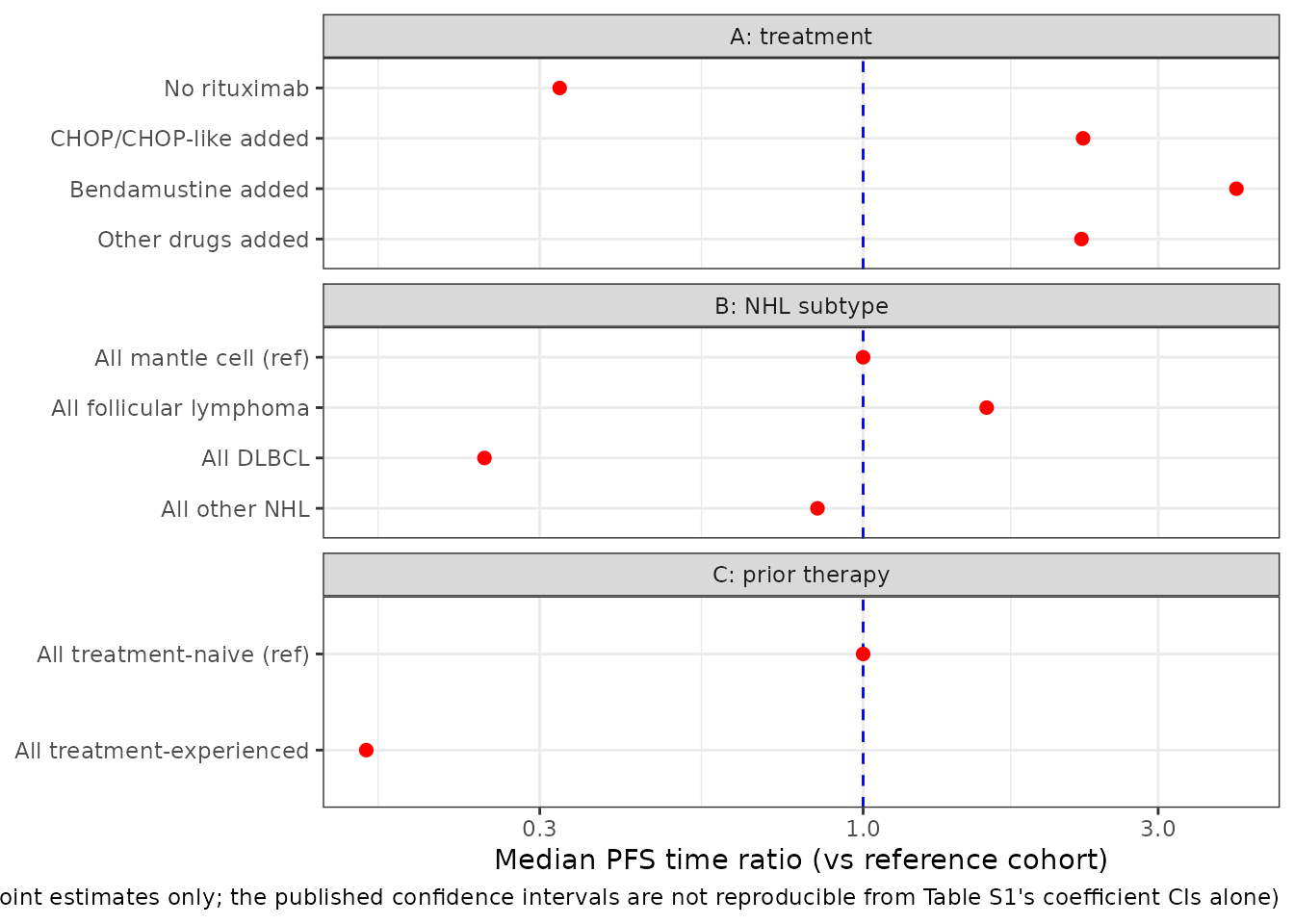
Replication of Li 2017 Figure 2 (visual predictive check)
Figure 2 of Li 2017 is a visual predictive check of cohort-level %PFS against time in months, with the observed 10th, 50th and 90th percentiles across cohorts. The digitised observations are not publicly available, so the panel below is the model’s own predictive distribution over a virtual database of 155 cohorts whose treatment, histology and prior-therapy mix matches Li 2017 Table 1. It reproduces the qualitative shape of the published figure: a steep early drop driven by the sub-1 Weibull shape, followed by a long flat tail, with an extremely wide between-cohort spread.
rxode2::rxSetSeed(20260916)

n_vpc <- 155L
set.seed(20260916)
vpc_cohorts <- tibble(
  id = seq_len(n_vpc),
  # Table 1 treatment coverage, as independent Bernoulli draws at the
  # published per-level cohort prevalences.
  CONMED_RITUX          = rbinom(n_vpc, 1, 0.632),
  CONMED_CHOP           = rbinom(n_vpc, 1, 0.264),
  CONMED_BENDAMUSTINE   = rbinom(n_vpc, 1, 0.070),
  CONMED_NONCHEMO_OTHER = rbinom(n_vpc, 1, 0.387)
) |>
  # Histology: assign each cohort a Table 1 stratum, then convert to the
  # percentage columns. "Mixed" cohorts get an even split.
  mutate(
    stratum = sample(
      c("FL", "MCL", "DLBCL", "OTHER", "MIXED"), n_vpc, replace = TRUE,
      prob = c(0.284, 0.213, 0.316, 0.025, 0.161)
    ),
    TUMTP_FL_PCT = case_when(
      stratum == "FL" ~ 100, stratum == "MIXED" ~ 100 / 3, TRUE ~ 0
    ),
    TUMTP_DLBCL_PCT = case_when(
      stratum == "DLBCL" ~ 100, stratum == "MIXED" ~ 100 / 3, TRUE ~ 0
    ),
    TUMTP_OTHER_NHL_PCT = case_when(stratum == "OTHER" ~ 100, TRUE ~ 0),
    # Table 1 "Number of treatments": 33.5% of cohorts on 1 regimen are
    # treated here as first-line, the rest as relapsed / refractory.
    LINE_1L_PCT = ifelse(rbinom(n_vpc, 1, 0.335) == 1, 100, 0)
  ) |>
  select(-stratum)

vpc_grid <- c(0, seq(1, 120, by = 1))
vpc_sim <- rxode2::rxSolve(
  mod, vpc_cohorts |> tidyr::expand_grid(time = vpc_grid)
) |>
  as.data.frame()

stopifnot(
  nrow(vpc_sim) == n_vpc * length(vpc_grid),
  !anyNA(vpc_sim$sur),
  all(vpc_sim$sur >= 0), all(vpc_sim$sur <= 1)
)

vpc_q <- vpc_sim |>
  group_by(time) |>
  summarise(
    p10 = quantile(sur, 0.10),
    p50 = quantile(sur, 0.50),
    p90 = quantile(sur, 0.90),
    .groups = "drop"
  )

ggplot(vpc_q, aes(x = time)) +
  geom_ribbon(aes(ymin = p10, ymax = p90), fill = "steelblue", alpha = 0.25) +
  geom_line(aes(y = p50), colour = "red", linewidth = 1) +
  geom_line(aes(y = p10), colour = "blue") +
  geom_line(aes(y = p90), colour = "blue") +
  coord_cartesian(ylim = c(0, 1)) +
  labs(
    x = "Time (month)", y = "Progression free survival (fraction)",
    caption = "Replicates the layout of Figure 2 of Li 2017: model-predicted median (red) and 10th / 90th percentiles (blue) of cohort-level PFS across a 155-cohort virtual database. Observed data are not publicly available."
  ) +
  theme_bw()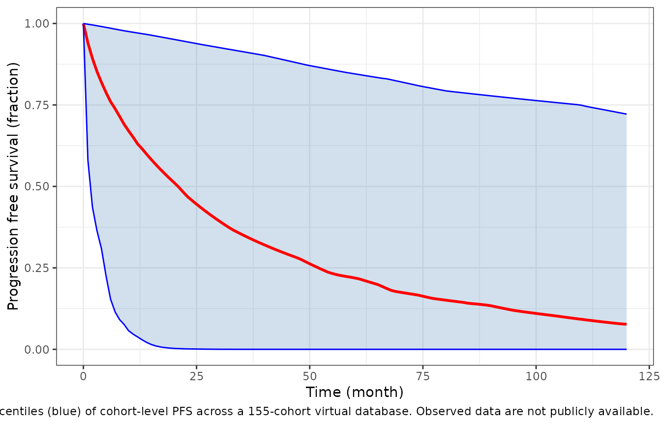
The predicted spread is deliberately wide: the between-study variance
on log(lambda) is 1.4, i.e. a standard deviation of 1.18 on
the log scale, so the central 95% of cohorts span a 114-fold range in
lambda after the covariates have been accounted for. That
is what the Figure 2 percentile bands look like in the published paper
too.
# The between-study spread is a structural property of omega, not of which
# cohorts happened to be drawn, so it is asserted on the model object
# rather than on the simulated sample.
stopifnot(
  abs(sqrt(diag(mod$omega)[["eta_study_llambda"]]) - sqrt(1.4)) < 1e-12,
  abs(sqrt(diag(mod$omega)[["eta_study_lk"]]) - sqrt(0.17)) < 1e-12
)

# The predicted median curve must be monotone and must stay inside the
# 10th-90th band; both are properties of the model, not of the draw.
stopifnot(
  all(diff(vpc_q$p50) <= 0),
  all(vpc_q$p50 >= vpc_q$p10), all(vpc_q$p50 <= vpc_q$p90)
)
Hazard-ratio scope
Li 2017 also validated the model against published hazard ratios
(100% of cohorts within 0.5- to 2-fold of the observed HR, 75% within
25%). Under a Weibull model two cohorts sharing the same shape
k have a time-constant hazard ratio equal to
(lambda_1 / lambda_2)^(-k), so a between-arm HR is
computable from this model directly. Because k itself
carries between-study variability, that identity only holds within a
study – which is exactly the comparison a randomised trial’s HR
makes.
hr_arms <- tibble(id = 1:2) |>
  mutate(
    CONMED_RITUX = 1, CONMED_CHOP = c(0, 1), CONMED_BENDAMUSTINE = 0,
    CONMED_NONCHEMO_OTHER = 0, TUMTP_FL_PCT = 0, TUMTP_DLBCL_PCT = 100,
    TUMTP_OTHER_NHL_PCT = 0, LINE_1L_PCT = 100
  )

hr_sim <- rxode2::rxSolve(
  rxode2::zeroRe(mod), hr_arms |> tidyr::expand_grid(time = c(6, 12, 24, 48))
) |>
  as.data.frame()
#> ℹ omega/sigma items treated as zero: 'eta_study_lk', 'eta_study_llambda'
#> Warning: multi-subject simulation without without 'omega'

hr <- hr_sim |>
  select(id, time, cumhaz, k, lambda) |>
  tidyr::pivot_wider(
    names_from = id, values_from = c(cumhaz, k, lambda)
  ) |>
  mutate(
    # The cumulative-hazard ratio of two same-shape Weibulls is constant.
    hr_cumhaz = cumhaz_2 / cumhaz_1,
    hr_closed = (lambda_2 / lambda_1)^(-k_1)
  )

stopifnot(
  nrow(hr) == 4L,
  !anyNA(hr$hr_cumhaz),
  # Time-constant, and equal to the closed form.
  diff(range(hr$hr_cumhaz)) < 1e-9,
  max(abs(hr$hr_cumhaz - hr$hr_closed)) < 1e-9,
  # Adding CHOP to a rituximab backbone must REDUCE the hazard.
  all(hr$hr_cumhaz < 1)
)
hr |>
  select(time, hr_cumhaz) |>
  rename("Time (month)" = time, "Hazard ratio, R-CHOP vs rituximab alone" = hr_cumhaz) |>
knitr::kable(digits = 4)| Time (month) | Hazard ratio, R-CHOP vs rituximab alone |
|---|---|
| 6 | 0.5236 |
| 12 | 0.5236 |
| 24 | 0.5236 |
| 48 | 0.5236 |
Assumptions and deviations
-
Residual error is stored UNWEIGHTED. The
Supplemental Content states the residual was “the standard error of
ln(-ln(PFS(t))), scaled by an estimated constant”. The per-observation residual SD is thereforeexpSd * SE_i, whereSE_iis the standard error of the cohort’s own transformed Kaplan-Meier estimate at that time point – a property of the digitised dataset (it depends on the number still at risk) that Li 2017 does not print a formula for.expSdin the model file is the unweighted scalarsqrt(1.2); downstream simulation code must multiply it bySE_i. This follows the library’s ratified convention for MBMA models whose observation weight touches only the residual (see theN_ARMregister entry and theMercier_2014_tramadol_tapentadol_mbma/Chen_2025_methotrexate_*_mbmaprecedent). Li 2017’s between-study etas are not SE-weighted, so no weighting column is needed insidemodel(). -
The residual is encoded as log-normal
(
~ lnorm()), not additive. A residual additive onln(-ln(PFS))is by construction additive onln(cumhaz), i.e. log-normal oncumhaz.cumhaz ~ lnorm(expSd)is therefore the source error model exactly, not an approximation of it. -
Both between-study etas are encoded as exponential
(log-scale). The source says only that “inter-study variability
was included on
lambdaandk” and the Table S1 footnote calls the numbers variances; it does not state the transform. The magnitudes force the log scale: an additive eta onlambdawith SDsqrt(1.4) = 1.18months against a 110-month scale is a 1% between-study spread, which cannot coexist with the cohort spread in Figure 2, and an additive eta onkwith SDsqrt(0.17) = 0.41againstk = 0.79would put roughly 3% of studies at an inadmissiblek < 0. The log scale also matches the exponential covariate model these same parameters carry. - Reference-population centering, not median centering. The Supplemental Content says the exponential covariate model was “centered by the median covariate value”, but also states the reference population explicitly (rituximab only / MCL / 100% treatment-naive). The reference-population reading is implemented, because it is the only one under which Figure 3 places MCL and “All naive patients” exactly on the ratio = 1.0 line. The database medians are not reported for the retained covariates in any case.
-
cumhazcarries no epsilon offset ont, deliberately. The usual library idiom for an algebraic model that takes a log of time is((t + 1e-6) / lambda)^k, so the log stays finite att = 0. That idiom is wrong for a Weibull with a shape below 1, because a small offset raised to a small power is not small: atk = 0.24(well inside this model’s between-study distribution, sincek = 0.79 * exp(eta)with variance 0.17) andlambda = 10months,(1e-6 / 10)^0.24 = 0.021, a 2% drop in the survivor function at time zero. The exact form gives0^k = 0andsur(0) = 1identically. The price is that the observation scaleln(cumhaz)is-Infatt = 0; that is faithful, becauseln(-ln(PFS))is undefined whereverPFS = 1and the source’s own transformed dataset therefore cannot contain a time-zero record either. Place observation records att > 0. (rxSolve()floors thelnormprediction at.Machine$double.epsrather than returningNaN, so a stray time-zero row does not poison a solve.) - Confidence intervals are not reproducible. Table S1 gives a 95% CI per coefficient but no covariance matrix, so the Figure 3 error bars cannot be regenerated. The Figure 3 replication above plots point estimates only.
-
Covariate scale. The canonical
_PCTcolumns are percentages (0-100) while Li 2017’s coefficients are per unit fraction; the model divides by 100. Li 2017 Table 1 prints its aggregate covariates as fractions in 0-1, so a user transcribing the source dataset directly must multiply by 100 before supplying these columns. - The prior-therapy covariate is linear in a column the paper treats as a threshold. Li 2017’s final model carries a single continuous “% experienced patients” coefficient, while its own subanalysis found treatment-naive and one-prior-line cohorts indistinguishable and two-or-more-prior-line cohorts at under a tenth the median PFS time. The linear form is the source model’s; the subanalysis parameters are not tabulated anywhere and are not extracted.
-
The sensitivity analysis is not extracted. Table
S1’s second block reports a complete-covariate sensitivity analysis on
the 91 studies with no imputed covariates. Per the library’s policy of
replicating the authors’ model structure, robustness checks the authors
did not report as final are excluded. For reference, it moved
kto 0.69 (95% CI 0.47, 0.91) andlambdato 118 (95% CI 35.7, 200.3) – under 15%, as the paper states – but additionally retained treatment and tumor-subtype effects onkthat the final model eliminated, and moved the bendamustine coefficient from 1.39 to 0.526 and the follicular- lymphoma coefficient from +0.46 to -0.142 (RSE 103%). -
Bortezomib and other chemotherapy carry no
coefficient. Both were screened as their own treatment levels
and eliminated in backward elimination; Table S1 prints
---and Figure 3A places both exactly on the ratio = 1.0 line. A cohort receiving either is represented in this model by its other regimen components only. They are recorded incovariatesDataExcludedso the provenance of the screen is preserved. -
Screened-and-dropped demographic covariates. Median
age, sex distribution, prior rituximab exposure, performance status
>= 2 and disease stage >= III were all tested and none was
significant at P < 0.01; none has a published point estimate. All are
recorded in
covariatesDataExcluded. - Simulation scope is study-arm level. The random effects are between-STUDY, so the model simulates cohort-level PFS curves, median PFS times and between-arm hazard ratios. It does not simulate individual-patient event times, and a single solve is one trial arm, not one patient.
- The virtual cohort in the Figure 2 replication is constructed, not published. Li 2017 Table 1 gives marginal cohort prevalences for each treatment and histology level but not their joint distribution, so the 155-cohort database above draws the treatment indicators independently at the published marginals and assigns histology strata by the published proportions. It is a plausibility panel, not a reproduction of the paper’s own predictive distribution.
Errata
Supplemental Content, Model Description, equation (1) is
defective as published. The supplement ships the equation as a
241 x 19 pixel raster image (word/media/image1.png inside
medi-96-e7988-s001.docx; the document contains no OMML and
no MathType object, so no higher-resolution original exists). Magnified,
that image reads
ln(-ln(PFS(t))) = k * ln(t) - k * ln(t)whose right-hand side is identically zero. The lambda of
the second term was lost in typesetting. The intended equation is the
standard Weibull probability-plot linearisation
ln(-ln(PFS(t))) = k * ln(t) - k * ln(lambda)equivalently PFS(t) = exp(-(t/lambda)^k), which is what
this model implements. Three independent checks fix that reading and
exclude the mirror image k*ln(lambda) - k*ln(t):
- The mirror image gives a survivor function
increasing in
t(PFS -> 1ast -> infinity), which is inadmissible and contradicts the monotone-decreasing visual predictive check in Li 2017 Figure 2. The monotonicity gate above is the assertion that would fail. - The supplement’s own text defines
lambdaas “the scale parameter” andkas “the shape parameter (also known as the Weibull slope)”. “Weibull slope” names the coefficient ofln tin precisely this linearisation, sokmust multiply+ln(t). - Under this reading the median PFS time is
lambda * ln(2)^(1/k), proportional tolambda, which is what makes every Table S1 coefficient exponentiate to the median-PFS-time ratio plotted in Figure 3. All ten Figure 3 entries reproduce to machine precision in the covariate gate above; under any other reading of the equation they would not.
No parameter value was tuned or back-solved to reach this conclusion.
No erratum or corrigendum was located for Li 2017 on the journal’s landing page or in PubMed; the only correction-shaped artefact is the equation raster described above, which is a typesetting loss in the supplement rather than a published correction.
The supplement’s backward-elimination narrative disagrees with its own Table S1 on one word. The Model Description says “Treatment (bortezomib, other drugs) on lambda … were removed in the backward elimination steps”, but Table S1’s final-model column carries “Other drugs on lambda” = 0.813 (RSE 8%, 95% CI 0.69 to 0.94), and both the Abstract (“other nonchemotherapy drugs, aside from bortezomib, prolonged median PFS time 2 to 4-fold”) and Figure 3A place “Other drugs” well above 1.0 and “Other chemo” exactly at 1.0. The parenthetical evidently means “(bortezomib, other chemotherapy)”. Table S1 and Figure 3A govern, and the model retains the other-drugs effect and drops bortezomib and other chemotherapy.