Biologics and small molecules for psoriasis: PASI75 and PASI90 MBMA (He 2021)
Source:vignettes/articles/He_2021_psoriasis_mbma.Rmd
He_2021_psoriasis_mbma.RmdModel and source
He H, Wu W, Zhang Y, Zhang M, Sun N, Zhao L, Wang X. Model-Based Meta-Analysis in Psoriasis: A Quantitative Comparison of Biologics and Small Targeted Molecules. Front Pharmacol. 2021;12:586827. doi:10.3389/fphar.2021.586827.
He 2021 is a longitudinal model-based meta-analysis (MBMA) of 17 systemic agents for moderate-to-severe plaque psoriasis. It fits two independent models with the same structure, one per end point, and this package ships each as its own model file:
-
He_2021_psoriasis_pasi75_mbma– the proportion of patients reaching a 75% reduction from baseline PASI (PASI75), 17 drugs (Table 2 and Supplementary Table S1). -
He_2021_psoriasis_pasi90_mbma– the same for a 90% reduction (PASI90), 16 drugs; alefacept had too few PASI90 data (Table 4 and Supplementary Table S2).
The structure follows the methodology of Checchio 2017
(Checchio_2017_psoriasis_pasi75_longitudinal_mbma), which
He 2021 cites for it. The logit of the responder rate is a placebo term
that rises exponentially to a plateau plus, for each drug, an Emax
dose-response multiplied by an exponential onset. Body weight acts on
the placebo plateau.
mod75 <- readModelDb("He_2021_psoriasis_pasi75_mbma")
mod90 <- readModelDb("He_2021_psoriasis_pasi90_mbma")
ui75 <- rxode2::rxode2(mod75)
ui90 <- rxode2::rxode2(mod90)
Population
Both models operate at the study-arm level: one observation is one trial arm’s responder proportion at one time, not one patient’s outcome. The random effect is between-study, and neither model may be used to simulate individual patients.
The dataset is 80 randomised placebo- or active-controlled trials, 235 treatment arms and 40,323 patients, identified from PubMed, Cochrane, Embase and ClinicalTrials.gov up to 18 July 2019 (Methods ‘Database Development’; Results ‘Characteristics of Included Studies’). PASI75 was reported in 233 arms and PASI90 in 224. Arm-level demographics are summarised as medians (range) in Table 1: 69.05% male, body weight 89.6 kg (66.6-99), age 45 years (38.6-55.3), baseline PASI 20 (11-33.1).
pop <- mod75()$population
tibble::tibble(
  Field = c("Species", "Trials", "Patients", "Arms (PASI75 / PASI90)",
            "Disease state", "Weight", "Female (%)"),
  Value = c(pop$species, pop$n_studies, pop$n_subjects, "233 / 224",
            pop$disease_state, pop$weight_range, pop$sex_female_pct)
) |>
knitr::kable()| Field | Value |
|---|---|
| Species | human |
| Trials | 80 |
| Patients | 40323 |
| Arms (PASI75 / PASI90) | 233 / 224 |
| Disease state | adults with moderate to severe plaque psoriasis in randomised placebo- or active-controlled trials; arm median baseline PASI 11-33.1 and body surface area involved 19-50.2% (Table 1) |
| Weight | arm median weights 66.6-99 kg (Table 1, ‘Total’ row: median 89.6 kg); predictions are made at 90 kg |
| Female (%) | 30.95 |
Source trace
Every model equation and parameter block, with where it came from. The in-file comments carry the same trace per parameter.
tibble::tribble(
  ~Component, ~Source,
  "N_response ~ binomial(N, P); P = inverse-logit(E0 + Edrug)", "Equations 1-3, Methods 'Model Development'",
  "E0 = BSL + A * (1 - exp(-kpbo * time * exp(eta)))", "Equation 4 (eta inside the exponent; see Assumptions)",
  "Edrug = Emax * (1 - exp(-k * time)) * dose / (dose + ED50)", "Equation 5, Hill coefficient c fixed to 1 per Methods",
  "ED50 = 0 FIX makes dose / (dose + ED50) = 1: written as (dose > 0)", "Results; Table 2 and Table 4 '0 FIX' entries",
  "Obs = P + Weight * eps; Weight = sqrt(P * (1 - P) / N)", "Equations 7-8",
  "A_i = A * (WT / 90)^theta", "Equation 9; 90 kg per the Figure 2-4 captions"
) |>
knitr::kable(caption = "Structural, covariate and residual equations.")| Component | Source |
|---|---|
| N_response ~ binomial(N, P); P = inverse-logit(E0 + Edrug) | Equations 1-3, Methods ‘Model Development’ |
| E0 = BSL + A * (1 - exp(-kpbo * time * exp(eta))) | Equation 4 (eta inside the exponent; see Assumptions) |
| Edrug = Emax * (1 - exp(-k * time)) * dose / (dose + ED50) | Equation 5, Hill coefficient c fixed to 1 per Methods |
| ED50 = 0 FIX makes dose / (dose + ED50) = 1: written as (dose > 0) | Results; Table 2 and Table 4 ‘0 FIX’ entries |
| Obs = P + Weight * eps; Weight = sqrt(P * (1 - P) / N) | Equations 7-8 |
| A_i = A * (WT / 90)^theta | Equation 9; 90 kg per the Figure 2-4 captions |
tibble::tribble(
  ~Model, ~Parameters, ~Source,
  "PASI75", "BSL, A, kpbo, weight effect on A, omega, sigma", "Supplementary Table S1",
  "PASI75", "Emax, ED50, k for 17 drugs (ED50 0 FIX for risankizumab, alefacept, methotrexate; apremilast Emax 9 FIX)", "Table 2",
  "PASI90", "BSL, A, kpbo, weight effect on A, omega, sigma", "Supplementary Table S2",
  "PASI90", "Emax, ED50, k for 16 drugs (ED50 0 FIX for ustekinumab, methotrexate; apremilast Emax 8.8 FIX)", "Table 4"
) |>
knitr::kable(caption = "Parameter provenance by block.")| Model | Parameters | Source |
|---|---|---|
| PASI75 | BSL, A, kpbo, weight effect on A, omega, sigma | Supplementary Table S1 |
| PASI75 | Emax, ED50, k for 17 drugs (ED50 0 FIX for risankizumab, alefacept, methotrexate; apremilast Emax 9 FIX) | Table 2 |
| PASI90 | BSL, A, kpbo, weight effect on A, omega, sigma | Supplementary Table S2 |
| PASI90 | Emax, ED50, k for 16 drugs (ED50 0 FIX for ustekinumab, methotrexate; apremilast Emax 8.8 FIX) | Table 4 |
The three display equations that carry the model (4, 5 and 9) are
typeset as images in the published PDF and are lost by a plain-text
conversion; they were read from the PDF’s text layer, and the position
of exp(eta) in Equation 4 was checked from the glyph
positions (it sits on the superscript baseline with -kpbo,
i.e. inside the exponent).
Regimens
Both models take dose through one
CONMED_<drug>_DOSE covariate column per drug and zero
in every other column. The value is the maintenance dose per
administration (mg; infliximab mg/kg). The regimens below are
the rows of Tables 3 and 5; the loading doses in their labels do not
enter the model.
doseCols <- c(
  "CONMED_ADALIMUMAB_DOSE", "CONMED_INFLIXIMAB_DOSE", "CONMED_ETANERCEPT_DOSE",
  "CONMED_CERTOLIZUMAB_DOSE", "CONMED_USTEKINUMAB_DOSE", "CONMED_BRIAKINUMAB_DOSE",
  "CONMED_GUSELKUMAB_DOSE", "CONMED_TILDRAKIZUMAB_DOSE", "CONMED_RISANKIZUMAB_DOSE",
  "CONMED_SECUKINUMAB_DOSE", "CONMED_IXEKIZUMAB_DOSE", "CONMED_BRODALUMAB_DOSE",
  "CONMED_APREMILAST_DOSE", "CONMED_TOFACITINIB_DOSE", "CONMED_BARICITINIB_DOSE",
  "CONMED_ALEFACEPT_DOSE", "CONMED_MTX_DOSE"
)

arms <- tibble::tribble(
  ~arm,                    ~regimen,                     ~col,                        ~dose, ~cls,
  "Adalimumab",            "80 mg wk 0, 40 mg q2w",      "CONMED_ADALIMUMAB_DOSE",       40, "TNF-alpha",
  "Infliximab",            "5 mg/kg wk 0, 2, 6, q8w",    "CONMED_INFLIXIMAB_DOSE",        5, "TNF-alpha",
  "Etanercept",            "50 mg biw",                  "CONMED_ETANERCEPT_DOSE",       50, "TNF-alpha",
  "Certolizumab pegol",    "400 mg wk 0, 2, 4, 200 mg q2w", "CONMED_CERTOLIZUMAB_DOSE", 200, "TNF-alpha",
  "Ustekinumab",           "45 mg wk 0, 4, q12w",        "CONMED_USTEKINUMAB_DOSE",      45, "IL-12/23",
  "Briakinumab",           "100 mg q4w",                 "CONMED_BRIAKINUMAB_DOSE",     100, "IL-12/23",
  "Guselkumab",            "100 mg wk 0, 4, q8w",        "CONMED_GUSELKUMAB_DOSE",      100, "IL-23",
  "Tildrakizumab",         "100 mg wk 0, 4, q12w",       "CONMED_TILDRAKIZUMAB_DOSE",   100, "IL-23",
  "Risankizumab",          "150 mg wk 0, 4, q12w",       "CONMED_RISANKIZUMAB_DOSE",    150, "IL-23",
  "Secukinumab",           "300 mg wk 0-4, q4w",         "CONMED_SECUKINUMAB_DOSE",     300, "IL-17",
  "Ixekizumab 160",        "160 mg wk 0, q4w",           "CONMED_IXEKIZUMAB_DOSE",      160, "IL-17",
  "Ixekizumab 80",         "160 mg wk 0, 80 mg q4w",     "CONMED_IXEKIZUMAB_DOSE",       80, "IL-17",
  "Brodalumab",            "210 mg wk 0, 1, 2, q2w",     "CONMED_BRODALUMAB_DOSE",      210, "IL-17",
  "Apremilast",            "30 mg b.i.d.",               "CONMED_APREMILAST_DOSE",       30, "PDE4",
  "Tofacitinib 5",         "5 mg b.i.d.",                "CONMED_TOFACITINIB_DOSE",       5, "JAK",
  "Tofacitinib 10",        "10 mg b.i.d.",               "CONMED_TOFACITINIB_DOSE",      10, "JAK",
  "Baricitinib",           "10 mg qd",                   "CONMED_BARICITINIB_DOSE",      10, "JAK",
  "Alefacept",             "10 mg qw",                   "CONMED_ALEFACEPT_DOSE",        10, "CD2",
  "Methotrexate",          "20 mg qw",                   "CONMED_MTX_DOSE",              20, "DHFR"
)

#' Build an rxode2 input frame: one id per arm, observations at `times`.
#' Only the dose columns the model uses are kept, so the PASI90 frame carries
#' no alefacept column.
makeArmData <- function(armTbl, times, cols, wt = 90, nArm = 100) {
  do.call(rbind, lapply(seq_len(nrow(armTbl)), function(i) {
    d <- data.frame(id = i, time = times, WT = wt, N_ARM = nArm)
    for (cc in cols) d[[cc]] <- 0
    d[[armTbl$col[i]]] <- armTbl$dose[i]
    d
  }))
}

arms90 <- arms |> filter(arm != "Alefacept")
cols90 <- setdiff(doseCols, "CONMED_ALEFACEPT_DOSE")

arms |>
  select(Regimen = arm, `Table 3/5 regimen` = regimen, `Dose column` = col,
         `Dose value` = dose) |>
knitr::kable(caption = "Regimens of He 2021 Tables 3 and 5 and the maintenance dose each maps to.")| Regimen | Table 3/5 regimen | Dose column | Dose value |
|---|---|---|---|
| Adalimumab | 80 mg wk 0, 40 mg q2w | CONMED_ADALIMUMAB_DOSE | 40 |
| Infliximab | 5 mg/kg wk 0, 2, 6, q8w | CONMED_INFLIXIMAB_DOSE | 5 |
| Etanercept | 50 mg biw | CONMED_ETANERCEPT_DOSE | 50 |
| Certolizumab pegol | 400 mg wk 0, 2, 4, 200 mg q2w | CONMED_CERTOLIZUMAB_DOSE | 200 |
| Ustekinumab | 45 mg wk 0, 4, q12w | CONMED_USTEKINUMAB_DOSE | 45 |
| Briakinumab | 100 mg q4w | CONMED_BRIAKINUMAB_DOSE | 100 |
| Guselkumab | 100 mg wk 0, 4, q8w | CONMED_GUSELKUMAB_DOSE | 100 |
| Tildrakizumab | 100 mg wk 0, 4, q12w | CONMED_TILDRAKIZUMAB_DOSE | 100 |
| Risankizumab | 150 mg wk 0, 4, q12w | CONMED_RISANKIZUMAB_DOSE | 150 |
| Secukinumab | 300 mg wk 0-4, q4w | CONMED_SECUKINUMAB_DOSE | 300 |
| Ixekizumab 160 | 160 mg wk 0, q4w | CONMED_IXEKIZUMAB_DOSE | 160 |
| Ixekizumab 80 | 160 mg wk 0, 80 mg q4w | CONMED_IXEKIZUMAB_DOSE | 80 |
| Brodalumab | 210 mg wk 0, 1, 2, q2w | CONMED_BRODALUMAB_DOSE | 210 |
| Apremilast | 30 mg b.i.d. | CONMED_APREMILAST_DOSE | 30 |
| Tofacitinib 5 | 5 mg b.i.d. | CONMED_TOFACITINIB_DOSE | 5 |
| Tofacitinib 10 | 10 mg b.i.d. | CONMED_TOFACITINIB_DOSE | 10 |
| Baricitinib | 10 mg qd | CONMED_BARICITINIB_DOSE | 10 |
| Alefacept | 10 mg qw | CONMED_ALEFACEPT_DOSE | 10 |
| Methotrexate | 20 mg qw | CONMED_MTX_DOSE | 20 |
Reproducing Table 3 (PASI75) and Table 5 (PASI90)
Tables 3 and 5 report, for a 90 kg arm at each regimen, the median PASI75 and PASI90 responder rate over 1,000 simulations at Weeks 4, 8, 12, 16 and 24. These are predictions, not parameter estimates, so reproducing them is an independent check on the whole encoding: 95 PASI75 cells and 90 PASI90 cells.
# zeroRe() removes every random effect on purpose, so rxode2's 'no sigma' and
# 'multi-subject simulation without omega' warnings are expected here.
weeks <- c(4, 8, 12, 16, 24)
tGrid <- sort(unique(c(seq(0, 24, by = 0.25), weeks)))
sol75 <- rxode2::rxSolve(rxode2::zeroRe(ui75), makeArmData(arms, tGrid, doseCols),
                         returnType = "data.frame") |>
  mutate(arm = arms$arm[id])
sol90 <- rxode2::rxSolve(rxode2::zeroRe(ui90), makeArmData(arms90, tGrid, cols90),
                         returnType = "data.frame") |>
  mutate(arm = arms90$arm[id])
# He 2021 Table 3, medians (%), transcribed.
table3 <- tibble::tribble(
  ~arm,                  ~w4,   ~w8,   ~w12,  ~w16,  ~w24,
  "Adalimumab",          21.30, 56.95, 67.80, 71.20, 72.80,
  "Infliximab",          34.10, 67.10, 75.65, 78.20, 79.70,
  "Etanercept",           7.98, 34.40, 49.60, 55.00, 57.80,
  "Certolizumab pegol",  15.30, 53.15, 67.70, 71.80, 74.00,
  "Ustekinumab",         10.75, 47.30, 65.30, 71.20, 74.50,
  "Briakinumab",         21.50, 66.80, 79.50, 82.80, 84.40,
  "Guselkumab",          20.65, 67.00, 80.40, 83.90, 85.80,
  "Tildrakizumab",        9.26, 42.80, 61.00, 68.10, 71.20,
  "Risankizumab",        21.15, 72.50, 85.95, 89.40, 91.00,
  "Secukinumab",         39.60, 77.20, 84.50, 86.70, 87.60,
  "Ixekizumab 160",      56.50, 80.40, 85.90, 87.70, 88.50,
  "Ixekizumab 80",       48.95, 75.20, 82.40, 84.60, 85.70,
  "Brodalumab",          48.55, 74.95, 81.70, 84.00, 85.20,
  "Apremilast",           5.68, 20.30, 29.50, 33.20, 35.30,
  "Tofacitinib 5",        9.07, 29.00, 39.20, 42.80, 45.10,
  "Tofacitinib 10",      16.30, 46.55, 57.70, 61.60, 63.10,
  "Baricitinib",          7.34, 33.10, 48.70, 54.80, 58.30,
  "Alefacept",            1.90,  7.46, 12.90, 15.90, 19.30,
  "Methotrexate",         4.14, 19.00, 30.80, 36.80, 40.10
)

# He 2021 Table 5, medians (%), transcribed.
table5 <- tibble::tribble(
  ~arm,                  ~w4,   ~w8,   ~w12,  ~w16,  ~w24,
  "Adalimumab",           6.10, 30.30, 43.50, 48.05, 50.60,
  "Infliximab",          10.40, 36.80, 49.15, 53.40, 55.90,
  "Etanercept",           1.16,  9.90, 22.00, 28.95, 34.40,
  "Certolizumab pegol",   2.29, 20.00, 36.50, 43.50, 47.80,
  "Ustekinumab",          2.64, 22.90, 41.60, 48.85, 53.30,
  "Briakinumab",          5.83, 37.10, 54.85, 60.80, 63.60,
  "Guselkumab",          11.70, 47.45, 61.00, 65.40, 67.40,
  "Tildrakizumab",        2.21, 18.10, 34.80, 40.70, 44.90,
  "Risankizumab",         5.11, 42.15, 65.50, 72.70, 76.70,
  "Secukinumab",         10.60, 47.95, 62.50, 66.70, 69.30,
  "Ixekizumab 160",      21.60, 55.35, 67.20, 71.10, 73.10,
  "Ixekizumab 80",       18.40, 50.40, 62.60, 66.95, 69.40,
  "Brodalumab",          19.90, 52.15, 64.50, 68.60, 70.80,
  "Apremilast",           0.38,  2.68,  6.09,  9.75, 16.40,
  "Tofacitinib 5",        1.99, 12.00, 19.50, 23.40, 25.10,
  "Tofacitinib 10",       3.52, 21.40, 33.60, 38.15, 40.70,
  "Baricitinib",          3.05, 17.20, 26.20, 29.95, 32.30,
  "Methotrexate",         0.85,  6.27, 13.05, 17.00, 20.10
)

#' Long-format comparison of a published table against the typical solve.
compareTable <- function(pub, sol, outcome) {
  pubLong <- pub |>
    pivot_longer(-arm, names_to = "week", values_to = "published") |>
    mutate(week = as.numeric(sub("w", "", week)))
  modLong <- sol |>
    filter(time %in% weeks) |>
    transmute(arm, week = time, model = 100 * .data[[outcome]])
  pubLong |>
    left_join(modLong, by = c("arm", "week")) |>
    mutate(diff = model - published)
}

cmp75 <- compareTable(table3, sol75, "prob_pasi75")
cmp90 <- compareTable(table5, sol90, "prob_pasi90")

cmp75 |>
  filter(week %in% c(4, 12, 24)) |>
  mutate(cell = sprintf("%.1f / %.1f", published, model)) |>
  select(arm, week, cell) |>
  pivot_wider(names_from = week, values_from = cell) |>
  rename(Regimen = arm, `Week 4 (pub / model)` = `4`,
         `Week 12 (pub / model)` = `12`, `Week 24 (pub / model)` = `24`) |>
knitr::kable(caption = "PASI75 (%) against He 2021 Table 3, 90 kg arm.")| Regimen | Week 4 (pub / model) | Week 12 (pub / model) | Week 24 (pub / model) |
|---|---|---|---|
| Adalimumab | 21.3 / 20.7 | 67.8 / 68.1 | 72.8 / 73.1 |
| Infliximab | 34.1 / 33.8 | 75.7 / 76.0 | 79.7 / 79.9 |
| Etanercept | 8.0 / 8.2 | 49.6 / 50.0 | 57.8 / 58.2 |
| Certolizumab pegol | 15.3 / 15.1 | 67.7 / 68.0 | 74.0 / 74.2 |
| Ustekinumab | 10.8 / 10.7 | 65.3 / 65.7 | 74.5 / 74.6 |
| Briakinumab | 21.5 / 21.4 | 79.5 / 79.9 | 84.4 / 84.6 |
| Guselkumab | 20.6 / 20.6 | 80.4 / 80.9 | 85.8 / 85.8 |
| Tildrakizumab | 9.3 / 9.3 | 61.0 / 61.7 | 71.2 / 71.6 |
| Risankizumab | 21.1 / 20.8 | 86.0 / 86.3 | 91.0 / 91.2 |
| Secukinumab | 39.6 / 39.9 | 84.5 / 84.9 | 87.6 / 87.7 |
| Ixekizumab 160 | 56.5 / 56.2 | 85.9 / 86.2 | 88.5 / 88.7 |
| Ixekizumab 80 | 49.0 / 49.8 | 82.4 / 82.8 | 85.7 / 85.8 |
| Brodalumab | 48.5 / 48.7 | 81.7 / 82.2 | 85.2 / 85.3 |
| Apremilast | 5.7 / 5.6 | 29.5 / 29.9 | 35.3 / 35.4 |
| Tofacitinib 5 | 9.1 / 9.2 | 39.2 / 39.7 | 45.1 / 45.4 |
| Tofacitinib 10 | 16.3 / 16.2 | 57.7 / 58.2 | 63.1 / 63.8 |
| Baricitinib | 7.3 / 7.1 | 48.7 / 48.9 | 58.3 / 58.6 |
| Alefacept | 1.9 / 1.9 | 12.9 / 13.0 | 19.3 / 19.6 |
| Methotrexate | 4.1 / 4.1 | 30.8 / 31.2 | 40.1 / 40.2 |
cmp90 |>
  filter(week %in% c(4, 12, 24)) |>
  mutate(cell = sprintf("%.1f / %.1f", published, model)) |>
  select(arm, week, cell) |>
  pivot_wider(names_from = week, values_from = cell) |>
  rename(Regimen = arm, `Week 4 (pub / model)` = `4`,
         `Week 12 (pub / model)` = `12`, `Week 24 (pub / model)` = `24`) |>
knitr::kable(caption = "PASI90 (%) against He 2021 Table 5, 90 kg arm.")| Regimen | Week 4 (pub / model) | Week 12 (pub / model) | Week 24 (pub / model) |
|---|---|---|---|
| Adalimumab | 6.1 / 6.0 | 43.5 / 44.1 | 50.6 / 51.1 |
| Infliximab | 10.4 / 10.6 | 49.1 / 49.9 | 55.9 / 56.6 |
| Etanercept | 1.2 / 1.2 | 22.0 / 22.5 | 34.4 / 34.7 |
| Certolizumab pegol | 2.3 / 2.3 | 36.5 / 36.9 | 47.8 / 48.3 |
| Ustekinumab | 2.6 / 2.7 | 41.6 / 42.0 | 53.3 / 53.9 |
| Briakinumab | 5.8 / 5.8 | 54.9 / 55.9 | 63.6 / 64.2 |
| Guselkumab | 11.7 / 11.7 | 61.0 / 61.6 | 67.4 / 67.9 |
| Tildrakizumab | 2.2 / 2.3 | 34.8 / 35.0 | 44.9 / 45.6 |
| Risankizumab | 5.1 / 5.1 | 65.5 / 66.3 | 76.7 / 76.9 |
| Secukinumab | 10.6 / 10.7 | 62.5 / 63.4 | 69.3 / 69.8 |
| Ixekizumab 160 | 21.6 / 22.2 | 67.2 / 68.2 | 73.1 / 73.7 |
| Ixekizumab 80 | 18.4 / 19.0 | 62.6 / 63.7 | 69.4 / 69.7 |
| Brodalumab | 19.9 / 20.4 | 64.5 / 65.5 | 70.8 / 71.3 |
| Apremilast | 0.4 / 0.4 | 6.1 / 6.5 | 16.4 / 16.7 |
| Tofacitinib 5 | 2.0 / 2.0 | 19.5 / 20.4 | 25.1 / 25.6 |
| Tofacitinib 10 | 3.5 / 3.5 | 33.6 / 34.4 | 40.7 / 41.4 |
| Baricitinib | 3.0 / 3.2 | 26.2 / 27.0 | 32.3 / 32.9 |
| Methotrexate | 0.8 / 0.8 | 13.1 / 13.4 | 20.1 / 20.4 |
# Deterministic comparison: the model side is a typical-value solve at the
# published parameters, the published side is fixed text. Nothing is drawn at
# random, so a tight bound over every cell is the right gate.
stopifnot(
  nrow(cmp75) == 95, !anyNA(cmp75$model),
  nrow(cmp90) == 90, !anyNA(cmp90$model),
  # PASI75 must be ~0 at randomisation: it is a reduction from each arm's own
  # baseline.
  all(sol75$prob_pasi75[sol75$time == 0] < 1e-3),
  max(abs(cmp75$diff)) < 1.0,
  max(abs(cmp90$diff)) < 1.5
)
cat(sprintf(
  "PASI75: max |model - Table 3| = %.2f pp over %d cells (mean signed %+.2f)\nPASI90: max |model - Table 5| = %.2f pp over %d cells (mean signed %+.2f)\n",
  max(abs(cmp75$diff)), nrow(cmp75), mean(cmp75$diff),
  max(abs(cmp90$diff)), nrow(cmp90), mean(cmp90$diff)
))
#> PASI75: max |model - Table 3| = 0.89 pp over 95 cells (mean signed +0.24)
#> PASI90: max |model - Table 5| = 1.30 pp over 90 cells (mean signed +0.53)
Every cell is reproduced to within 1 percentage point for PASI75 and 1.5 points for PASI90. The typical-value solve sits slightly above the published medians on average, more so for PASI90. That is expected rather than a transcription error: the published values are medians of 1,000 simulations that carry random effects and, going by the width of the reported intervals, parameter uncertainty, and those medians need not coincide with the typical-value prediction. The same selection of maintenance doses reproduces both tables, which is what settles the dose metric (see Assumptions).
Figures 2 and 4: time courses at the clinical dose
sol75 |>
  left_join(select(arms, arm, cls), by = "arm") |>
  ggplot(aes(time, 100 * prob_pasi75, colour = arm)) +
  geom_line(linewidth = 0.6) +
  facet_wrap(~cls) +
  labs(x = "Time (weeks)", y = "PASI75 responders (%)", colour = NULL) +
  coord_cartesian(ylim = c(0, 100)) +
  theme_bw() +
  theme(legend.position = "bottom")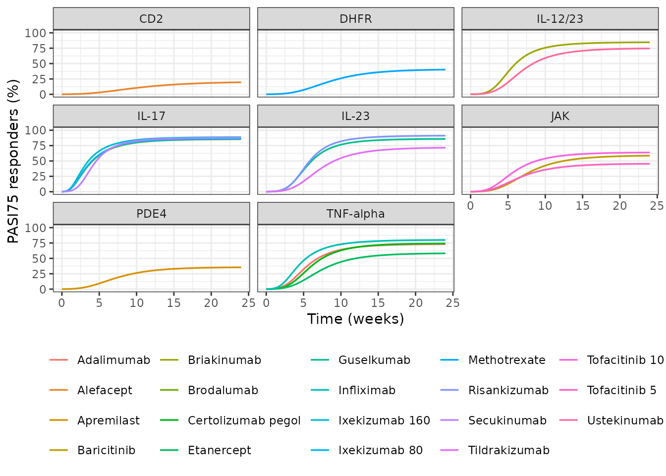
Replicates Figure 2 of He 2021: model-predicted typical PASI75 time course by regimen, 90 kg arm.
sol90 |>
  left_join(select(arms, arm, cls), by = "arm") |>
  ggplot(aes(time, 100 * prob_pasi90, colour = arm)) +
  geom_line(linewidth = 0.6) +
  facet_wrap(~cls) +
  labs(x = "Time (weeks)", y = "PASI90 responders (%)", colour = NULL) +
  coord_cartesian(ylim = c(0, 100)) +
  theme_bw() +
  theme(legend.position = "bottom")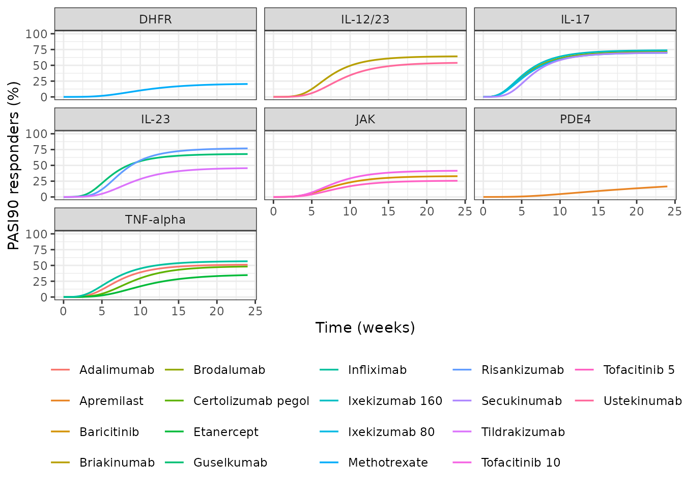
Replicates Figure 4 of He 2021: model-predicted typical PASI90 time course by regimen, 90 kg arm.
Figure 3: Week-12 ranking
rank12 <- bind_rows(
  cmp75 |> filter(week == 12) |> mutate(endpoint = "A: PASI75"),
  cmp90 |> filter(week == 12) |> mutate(endpoint = "B: PASI90")
)
rank12 |>
  mutate(arm = reorder(paste(arm, endpoint, sep = "___"), model)) |>
  ggplot(aes(model, arm)) +
  geom_point(colour = "black") +
  geom_point(aes(x = published), shape = 1, colour = "red", size = 2.5) +
  scale_y_discrete(labels = function(x) sub("___.*$", "", x)) +
  facet_wrap(~endpoint, scales = "free_y") +
  labs(x = "Week-12 responders (%): model (filled) and Table 3 / 5 (open)", y = NULL) +
  theme_bw()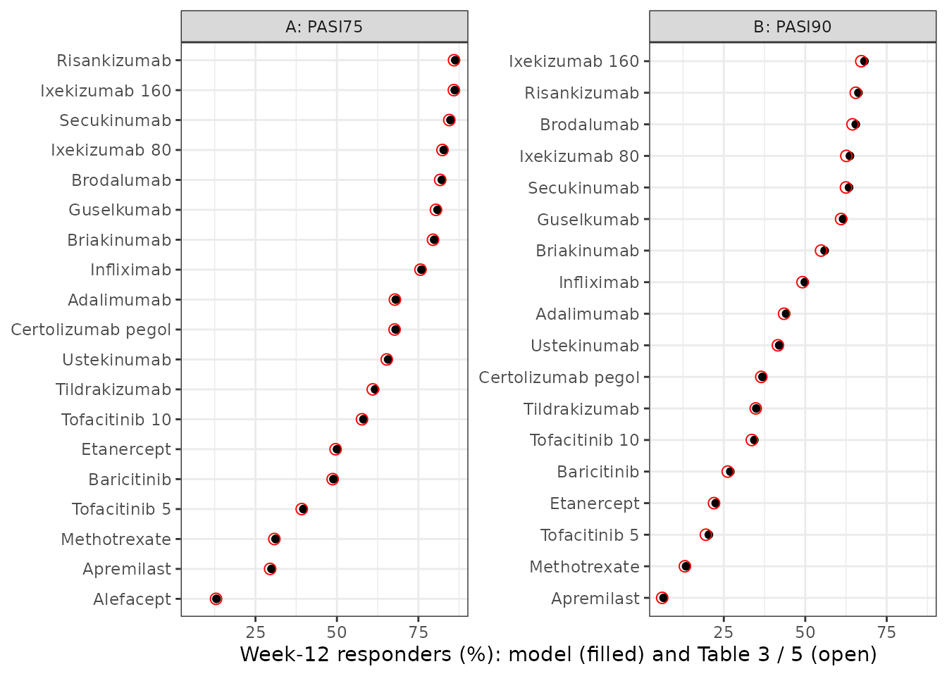
Replicates the median points of Figure 3 of He 2021: Week-12 PASI75 (A) and PASI90 (B) by regimen, typical 90 kg arm, ranked from high to low.
top75 <- rank12 |> filter(endpoint == "A: PASI75") |> arrange(desc(model))
top90 <- rank12 |> filter(endpoint == "B: PASI90") |> arrange(desc(model))
stopifnot(
  # Results: risankizumab then ixekizumab 160 mg lead PASI75 at Week 12, and
  # ixekizumab 160 mg then risankizumab lead PASI90.
  identical(top75$arm[1:2], c("Risankizumab", "Ixekizumab 160")),
  identical(top90$arm[1:2], c("Ixekizumab 160", "Risankizumab")),
  # Alefacept is the least efficacious PASI75 regimen and apremilast the least
  # efficacious PASI90 regimen.
  tail(top75$arm, 1) == "Alefacept",
  tail(top90$arm, 1) == "Apremilast"
)
The ordering statements in the Results – risankizumab then ixekizumab 160 mg at the top of the Week-12 PASI75 ranking, the reverse for PASI90, alefacept and apremilast at the bottom – all hold for the packaged models.
Where the between-study effect acts
Equation 4 prints the between-study random effect inside the
exponent, on the placebo onset rate:
exp(-kpbo * time * exp(eta)). Supplementary Tables S1 and
S2 label the same variance row omega(A), %, which would put
it on the asymptote A. The two readings give identical typical values,
so Tables 3 and 5 cannot separate them. The paper’s own visual
predictive check (Supplementary Figure S3) can. That figure is a vector
graphic, so its percentile lines were read exactly from the PDF’s
drawing coordinates. For the risankizumab panel (one regimen, ED50 fixed
to 0, so no dose mixing) they give:
vpcRis <- tibble::tribble(
  ~week, ~p025, ~p50, ~p975,
  4,       7.6, 21.5,  43.0,
  22,     84.0, 91.3,  99.1
)
knitr::kable(vpcRis, caption = "Risankizumab PASI75 VPC percentiles (%), Supplementary Figure S3, read from the vector drawing.")| week | p025 | p50 | p975 |
|---|---|---|---|
| 4 | 7.6 | 21.5 | 43.0 |
| 22 | 84.0 | 91.3 | 99.1 |
At Week 22 the placebo term has reached its plateau, so a random
effect on the onset rate barely moves the prediction, while one on the
asymptote moves it in full. The deterministic calculation below
evaluates the typical risankizumab arm with the random effect held at
its 2.5th and 97.5th percentiles (+/- 1.96 omega) under
each reading, with no residual error.
p75 <- setNames(ui75$iniDf$est, ui75$iniDf$name)
omega <- sqrt(p75[["eta_study_lkpbo"]])

#' Typical risankizumab PASI75 (%) at `t` weeks with the random effect `eta`
#' on the onset rate (`where = "kpbo"`) or on the asymptote (`where = "A"`).
risPasi75 <- function(t, eta, where) {
  kpbo <- exp(p75[["lkpbo"]] + if (where == "kpbo") eta else 0)
  asym <- p75[["asym_pbo"]] * if (where == "A") exp(eta) else 1
  e0 <- p75[["bsl_pbo"]] + asym * (1 - exp(-kpbo * t))
  ed <- p75[["emax_risankizumab"]] * (1 - exp(-exp(p75[["lkdrug_risankizumab"]]) * t))
  100 * stats::plogis(e0 + ed)
}

placement <- expand.grid(week = c(4, 22), where = c("kpbo", "A"),
                         stringsAsFactors = FALSE) |>
  rowwise() |>
  mutate(
    lo = risPasi75(week, -1.96 * omega, where),
    typical = risPasi75(week, 0, where),
    hi = risPasi75(week, 1.96 * omega, where)
  ) |>
  ungroup()

placement |>
  mutate(where = ifelse(where == "kpbo", "onset rate kpbo (Equation 4)", "asymptote A (table label)")) |>
  rename(Week = week, `Random effect on` = where, `2.5th (%)` = lo,
         `Typical (%)` = typical, `97.5th (%)` = hi) |>
knitr::kable(digits = 1, caption = "Spread of the risankizumab arm from the between-study effect alone.")| Week | Random effect on | 2.5th (%) | Typical (%) | 97.5th (%) |
|---|---|---|---|---|
| 4 | onset rate kpbo (Equation 4) | 10.3 | 20.8 | 37.4 |
| 22 | onset rate kpbo (Equation 4) | 89.8 | 91.0 | 91.2 |
| 4 | asymptote A (table label) | 7.6 | 20.8 | 63.4 |
| 22 | asymptote A (table label) | 61.8 | 91.0 | 99.5 |
wk22 <- placement |> filter(week == 22)
stopifnot(
  # On the asymptote, the effect alone pushes the Week-22 2.5th percentile far
  # below the VPC's 84.0%, before any residual error widens it further.
  wk22$lo[wk22$where == "A"] < 70,
  # On the onset rate, the effect has all but vanished by Week 22 (about one
  # percentage point either way).
  wk22$typical[wk22$where == "kpbo"] - wk22$lo[wk22$where == "kpbo"] < 2
)

# Arm size at which the residual alone (sigma = 1.33 times the binomial SE)
# places the 2.5th percentile at the VPC's 84.0%.
pTyp <- wk22$typical[wk22$where == "kpbo"] / 100
nImplied <- (1.96 * p75[["addSd_prob_pasi75"]] * sqrt(pTyp * (1 - pTyp)) / (pTyp - 0.840))^2
cat(sprintf("Residual-only reading of the Week-22 VPC band implies an arm size of about %.0f patients.\n", nImplied))
#> Residual-only reading of the Week-22 VPC band implies an arm size of about 113 patients.
Under the table’s label the between-study effect alone would put the Week-22 2.5th percentile at 62%, far outside the published band, and residual error could only widen it. Under Equation 4 the effect moves Week 22 by barely a percentage point and the band is residual error, which reproduces the VPC’s 84.0% lower line for arms of about 110 patients, a plausible arm size for the phase 2 and 3 risankizumab trials pooled in that panel. Both models therefore place the random effect as Equation 4 prints it.
Between-study variability
Simulating study arms rather than typical values shows the spread a trial designer should expect. The cohort is 150 risankizumab arms of 100 patients each (within the 200-per-arm cap), with the between-study effect and the residual error drawn; the lines of the Supplementary Figure S3 panel are overlaid.
rxode2::rxSetSeed(20210701)
nArms <- 150
bsvArms <- arms |> filter(arm == "Risankizumab") |> slice(rep(1, nArms))
bsvSol <- rxode2::rxSolve(ui75, makeArmData(bsvArms, 0:24, doseCols, nArm = 100),
                          returnType = "data.frame")

bsvQ <- bsvSol |>
  group_by(time) |>
  summarise(lo = stats::quantile(sim, 0.025), md = stats::median(sim),
            hi = stats::quantile(sim, 0.975), .groups = "drop")

ggplot(bsvQ, aes(time)) +
  geom_ribbon(aes(ymin = 100 * lo, ymax = 100 * hi), fill = "grey80") +
  geom_line(aes(y = 100 * md), linewidth = 0.8) +
  geom_point(data = pivot_longer(vpcRis, -week), aes(week, value), colour = "red") +
  labs(x = "Time (weeks)", y = "PASI75 responders (%)") +
  coord_cartesian(ylim = c(0, 100)) +
  theme_bw()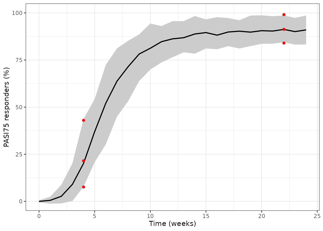
Simulated spread of 150 risankizumab 150 mg arms of 100 patients (grey: 2.5th-97.5th percentile of the simulated observations; black: median). Red points: the Supplementary Figure S3 VPC percentiles.
typRis <- sol75 |> filter(arm == "Risankizumab", time == 12)
stopifnot(
  # Central tendency only: the simulated extremes are not reproducible across
  # rxode2 builds.
  abs(100 * (bsvQ$md[bsvQ$time == 12] - typRis$prob_pasi75)) < 3,
  abs(100 * bsvQ$md[bsvQ$time == 22] - vpcRis$p50[vpcRis$week == 22]) < 3
)
Body weight
Body weight enters only the placebo asymptote, through a negative power (PASI75 -0.245, PASI90 -0.214), so heavier arms have a lower placebo plateau and, because the drug term adds on the same logit scale, a slightly lower total response.
# Typical-value solve; see the typical-sim chunk for the expected warnings.
wtDat <- bind_rows(lapply(c(70, 90, 110), function(w) {
  makeArmData(arms |> filter(arm == "Adalimumab"), 24, doseCols, wt = w) |>
    mutate(id = w)
}))
wtSol <- rxode2::rxSolve(rxode2::zeroRe(ui75), wtDat, returnType = "data.frame")
wtSol |>
  transmute(`Arm mean weight (kg)` = id, `Adalimumab Week-24 PASI75 (%)` = 100 * prob_pasi75) |>
knitr::kable(digits = 1)| Arm mean weight (kg) | Adalimumab Week-24 PASI75 (%) |
|---|---|
| 70 | 78.7 |
| 90 | 73.1 |
| 110 | 68.3 |
NCA
These models have no pharmacokinetic layer: dose enters as a covariate, there are no dose events and no concentrations, so a non-compartmental analysis does not apply. The validation above compares the models against every predicted value the paper publishes instead.
Assumptions and deviations
Dose is the per-administration maintenance dose
Tables 1, 3 and 5 give regimens, not the number the model reads. The dose metric is settled by the published predictions: ixekizumab 160 mg and 80 mg maintenance share one parameter set and are reproduced only by Dose = 160 and 80; tofacitinib 5 and 10 mg b.i.d. only by Dose = 5 and 10 (not the daily totals); apremilast 30 mg b.i.d. by Dose = 30 (Dose = 60 gives a Week-12 PASI75 of 61% against a published 29.5%); adalimumab by the 40 mg maintenance dose, not the 80 mg loading dose (83% against 67.8%). The Results text says the same for adalimumab (“the clinical dosage is 40 mg every 2 weeks”). Certolizumab pegol’s ‘400 mg 0, 2, 4, 200 mg q2w’ row is closer with Dose = 200 (68.0% against 67.7%) than with 400 (70.0%). Infliximab is mg/kg.
# Typical-value solves; see the typical-sim chunk for the expected warnings.
alt <- tibble::tribble(
  ~arm,                 ~col,                       ~chosen, ~alternative, ~published,
  "Adalimumab",         "CONMED_ADALIMUMAB_DOSE",        40,           80,      67.80,
  "Certolizumab pegol", "CONMED_CERTOLIZUMAB_DOSE",     200,          400,      67.70,
  "Apremilast",         "CONMED_APREMILAST_DOSE",        30,           60,      29.50,
  "Tofacitinib 10",     "CONMED_TOFACITINIB_DOSE",       10,           20,      57.70
)
#' Week-12 typical PASI75 (%) for one drug column at one dose.
wk12At <- function(col, dose) {
  d <- makeArmData(tibble::tibble(col = col, dose = dose), 12, doseCols)
  100 * rxode2::rxSolve(rxode2::zeroRe(ui75), d, returnType = "data.frame")$prob_pasi75
}
alt <- alt |>
  rowwise() |>
  mutate(modelChosen = wk12At(col, chosen), modelAlternative = wk12At(col, alternative)) |>
  ungroup()
alt |>
  select(Regimen = arm, `Table 3 Week 12 (%)` = published,
         `Dose used` = chosen, `Model (%)` = modelChosen,
         `Alternative dose` = alternative, `Model at alternative (%)` = modelAlternative) |>
knitr::kable(digits = 1)| Regimen | Table 3 Week 12 (%) | Dose used | Model (%) | Alternative dose | Model at alternative (%) |
|---|---|---|---|---|---|
| Adalimumab | 67.8 | 40 | 68.1 | 80 | 83.0 |
| Certolizumab pegol | 67.7 | 200 | 68.0 | 400 | 70.0 |
| Apremilast | 29.5 | 30 | 29.9 | 60 | 60.9 |
| Tofacitinib 10 | 57.7 | 10 | 58.2 | 20 | 71.1 |
Where the between-study random effect acts
Equation 4 places exp(eta) on the placebo onset rate;
Supplementary Tables S1 and S2 label the variance omega(A).
The equation is followed, because the paper’s own VPC is incompatible
with the table label (see “Where the between-study effect acts”).
Typical-value predictions are unaffected either way.
Random-effect and residual scale
The random effect is printed as a CV (24.9% for PASI75, 26% for
PASI90) and is converted to a log-normal variance by
log(1 + CV^2) (0.0602 and 0.0654). Reading the CV instead
as sqrt(omega^2) gives 0.0620 and 0.0676, an immaterial
difference. The residual term is printed as sigma = 1.33 in
both tables and is read as a standard deviation, the symbol the Methods
use for the square root of the residual variance; the variance reading
would give 1.153. Either way it multiplies the binomial standard error
sqrt(P(1 - P)/N), so simulating it needs the arm size in an
N_ARM column.
Body weight centring
Equation 9 divides by “mean(covariate)” without a number. 90 kg is used: the captions of Figures 2-4 call 90 kg the average body weight, all published predictions are made at 90 kg, and the Table 1 dataset median is 89.6 kg (which would change the weight factor by 0.1%). Arms that did not report weight were set to the dataset median by the authors; downstream users should do the same.
ED50 fixed at zero
Where the authors fixed an ED50 to 0 (PASI75: risankizumab,
alefacept, methotrexate; PASI90: ustekinumab, methotrexate),
dose / (dose + 0) is 1 for every positive dose, so the
model reads only whether the dose column is positive. No log-scale ED50
parameter is declared for these drugs because a log scale cannot hold 0.
For those drugs the model predicts the response at the doses studied and
nothing about other doses. Risankizumab and ustekinumab differ between
the two models in this respect, exactly as in the paper.