IPSS in benign prostatic hyperplasia: tamsulosin, dutasteride and combination (D'Agate 2020)
Source:vignettes/articles/DAgate_2020_bph_ipss_mbma.Rmd
DAgate_2020_bph_ipss_mbma.RmdModel and source
ui <- rxode2::rxode(readModelDb("DAgate_2020_bph_ipss_mbma"))
#> ℹ parameter labels from comments will be replaced by 'label()'
#> Warning: some etas defaulted to non-mu referenced, possible parsing error: etaldisp, etaldelta_pbo
#> as a work-around try putting the mu-referenced expression on a simple line- Citation: D’Agate S, Wilson T, Adalig B, Manyak M, Palacios-Moreno JM, Chavan C, Oelke M, Roehrborn C, Della Pasqua O. Model-based meta-analysis of individual International Prostate Symptom Score trajectories in patients with benign prostatic hyperplasia with moderate or severe symptoms. Br J Clin Pharmacol. 2020;86(8):1585-1599. doi:10.1111/bcp.14268. Parameter values from Tables 2 and 3; structural equation, covariate functional forms and the placebo random-effect block from the NONMEM control stream in the Supporting Information appendix.
- Article: https://doi.org/10.1111/bcp.14268
- Supplement (Supporting Information, including the final NONMEM control stream as an appendix): https://doi.org/10.1111/bcp.14268
D’Agate 2020 is an individual-patient-data model-based meta-analysis of six phase III/IV dutasteride trials (ARIA3001, ARIA3002, ARI40002, CombAT, CONDUCT, ARIB3003; 10,238 men, 140,733 IPSS observations, up to 4 years). It describes the time course of the International Prostate Symptom Score (IPSS, 0-35) with one ordinary differential equation (Equations 1-3):
The first term is a zero-order worsening of symptoms (the disease
progression rate DISP) that shuts off as the score
approaches the scale maximum of 35. The second term is a first-order
improvement: a placebo effect that wears off with a 7.3-month half-life,
plus a constant effect for the active treatment (tamsulosin,
dutasteride, watchful waiting, or tamsulosin-dutasteride combination
therapy).
Population
str(ui$population)
#> List of 11
#>  $ species       : chr "human"
#>  $ n_subjects    : int 10238
#>  $ n_studies     : int 6
#>  $ age_range     : chr "47-94 years (median 66, mean 66.2)"
#>  $ weight_range  : chr "37-179 kg (median 82, mean 83.2)"
#>  $ sex_female_pct: num 0
#>  $ race_ethnicity: chr "white 9268, black 229, Hispanic 276, Asian 374 (Table 1)"
#>  $ disease_state : chr "Men with moderate or severe LUTS due to BPH; baseline IPSS median 16 (range 1-35), prostate volume median 48.6 "| __truncated__
#>  $ dose_range    : chr "Placebo (n = 2158, 2 y); watchful waiting with protocol-defined tamsulosin initiation (n = 373); tamsulosin 0.4"| __truncated__
#>  $ regions       : chr "multinational"
#>  $ notes         : chr "Studies ARIA3001, ARIA3002, ARI40002, CombAT, CONDUCT and ARIB3003; 140,733 IPSS observations (Methods 2.1, Tab"| __truncated__
Table 1 of the paper: men aged 47-94 years (median 66), body weight median 82 kg, baseline IPSS median 16 (range 1-35; 66% moderate, 29% severe at the start of treatment), median prostate volume 48.6 cm^3, median PSA 3.4 ng/mL, median BPH symptom duration 4 years; predominantly white (9268 of 10,147 with race recorded). Placebo was given to 2158 men for 2 years; 373 were in the CONDUCT watchful-waiting arm, 1611 received tamsulosin 0.4 mg, 3790 dutasteride 0.5 mg and 2143 the combination, for up to 4 years.
Source trace
The control stream in the Supporting Information runs in days; Tables
2 and 3 report the same quantities per month. The conversion factor is
30 days/month: THETA(1) = 0.0116 /day x 30 = 0.348 (Table
2: 0.347), THETA(2) = 0.00202 /day x 30 = 0.0606 (Table 2:
0.061), THETA(3) = 218 days / 30 = 7.27 (Table 2: 7.263).
The model uses the Table 2 / Table 3 values directly, in months.
| Quantity | Model name | Value | Source |
|---|---|---|---|
| Structural ODE | d/dt(ipss) |
Eq. 1 | Eq. 1; control stream DADT(1)
|
| Placebo effect | eff_pbo |
Eq. 2 | Eq. 2; control stream EFFpl
|
| Treatment effect | eff_trt |
Eq. 3 | Eq. 3; control stream EFFtrt by ARM
|
| Initial condition | ipss(0) <- IPSS_BL |
observed baseline | control stream A_0(1) = obsIPSS
|
| DISP | ldisp |
0.347 points/month | Table 2 |
| DELTA placebo | ldelta_pbo |
0.061 /month | Table 2 |
| Placebo T1/2 | lthalf_pbo |
7.263 months | Table 2 |
| BPHDUR on placebo magnitude | e_t_sympt_bph_delta_pbo |
-0.025 /year, centred at 4 y | Table 2; linear form and centre from control stream
DELTpBPHDUR
|
| IPSSb on DISP | e_ipss_bl_disp |
0.027 /point, centred at 16 | Table 2; linear form and centre from control stream
DISPIPSS0
|
| Alcohol use on placebo T1/2 | e_alcohol_use_thalf_pbo |
-0.135 | Table 2; form from control stream T12pALCU
|
| DELTA tamsulosin | ldelta_tamsulosin |
0.015 /month | Table 3 |
| DELTA dutasteride | ldelta_dutasteride |
0.016 /month | Table 3 |
| DELTA watchful waiting | ldelta_ww |
0.018 /month | Table 3 |
| DELTA combination | ldelta_fdc |
0.032 /month | Table 3 |
| IIV DISP, placebo, T1/2 (variances) |
etaldisp, etaldelta_pbo,
etalthalf_pbo
|
0.997, 2.822, 2.758 | Table 2 |
| Correlations in the placebo block | off-diagonals | -0.544, 0.307, -0.965 | control stream $OMEGA BLOCK(3)
|
| IIV treatment effects (variances) | etaldelta_* |
tamsulosin 1.923, dutasteride 1.734, WW 1.812, combination 1.449 | Table 3 |
| Additive residual SD | addSd_* |
placebo 3.224, tamsulosin 3.613, dutasteride 3.506, WW 2.778, combination 3.141 | Tables 2 and 3 |
ini_df <- as.data.frame(ui$iniDf)
ini_df |>
  dplyr::filter(is.na(neta1)) |>
  dplyr::transmute(
    Parameter = name,
    Estimate = signif(ifelse(grepl("^l", name), exp(est), est), 4),
    Scale = ifelse(grepl("^l", name), "back-transformed", "as estimated"),
    Fixed = fix
  ) |>
knitr::kable(caption = "Fixed effects and residual SDs (log-scale parameters back-transformed).")| Parameter | Estimate | Scale | Fixed |
|---|---|---|---|
| ldisp | 0.347 | back-transformed | TRUE |
| ldelta_pbo | 0.061 | back-transformed | TRUE |
| lthalf_pbo | 7.263 | back-transformed | TRUE |
| e_t_sympt_bph_delta_pbo | -0.025 | as estimated | TRUE |
| e_ipss_bl_disp | 0.027 | as estimated | TRUE |
| e_alcohol_use_thalf_pbo | -0.135 | as estimated | TRUE |
| ldelta_tamsulosin | 0.015 | back-transformed | FALSE |
| ldelta_dutasteride | 0.016 | back-transformed | FALSE |
| ldelta_ww | 0.018 | back-transformed | FALSE |
| ldelta_fdc | 0.032 | back-transformed | FALSE |
| addSd_pbo | 3.224 | as estimated | TRUE |
| addSd_tamsulosin | 3.613 | as estimated | FALSE |
| addSd_dutasteride | 3.506 | as estimated | FALSE |
| addSd_ww | 2.778 | as estimated | FALSE |
| addSd_fdc | 3.141 | as estimated | FALSE |
Structural checks
Unit conversion between the control stream and the tables
unit_chk <- data.frame(
  quantity = c("DISP", "DELTA placebo", "placebo T1/2"),
  control_stream_per_day = c(0.0116, 0.00202, 218),
  converted_per_month = c(0.0116 * 30, 0.00202 * 30, 218 / 30),
  table2 = c(0.347, 0.061, 7.263)
)
unit_chk$pct_diff <- 100 * (unit_chk$converted_per_month / unit_chk$table2 - 1)
knitr::kable(unit_chk, digits = 4)| quantity | control_stream_per_day | converted_per_month | table2 | pct_diff |
|---|---|---|---|---|
| DISP | 0.0116 | 0.3480 | 0.347 | 0.2882 |
| DELTA placebo | 0.0020 | 0.0606 | 0.061 | -0.6557 |
| placebo T1/2 | 218.0000 | 7.2667 | 7.263 | 0.0505 |
Long-term steady state is closed-form
Once the placebo effect has decayed, a constant treatment effect
E gives DISP (1 - I/35) = E I, so the score
settles at I* = DISP / (E + DISP/35). Solving the
typical-value model for 100 years must land on that value.
mod_typ <- rxode2::zeroRe(ui)
#> Warning: No sigma parameters in the model
#> Warning: some etas defaulted to non-mu referenced, possible parsing error: etaldisp, etaldelta_pbo
#> as a work-around try putting the mu-referenced expression on a simple line

arm_cov <- function(arm) {
  data.frame(
    TRT_TAMSULOSIN = as.integer(arm == "Tamsulosin"),
    TRT_DUTASTERIDE = as.integer(arm == "Dutasteride"),
    TRT_TAMSULOSIN_DUTASTERIDE = as.integer(arm == "Combination"),
    TRT_WATCHFUL_WAITING = as.integer(arm == "Watchful waiting")
  )
}
arms <- c("Placebo", "Tamsulosin", "Dutasteride", "Combination", "Watchful waiting")

ss_ev <- do.call(rbind, lapply(seq_along(arms), function(i) {
  cbind(
    data.frame(id = i, time = c(0, 1200), evid = 0, cmt = "ipss",
               IPSS_BL = 16, T_SYMPT_BPH = 4, ALCOHOL_USE = 0),
    arm_cov(arms[i])
  )
}))
ss_sim <- as.data.frame(rxode2::rxSolve(mod_typ, ss_ev, returnType = "data.frame"))
#> ℹ omega/sigma items treated as zero: 'etaldisp', 'etaldelta_pbo', 'etalthalf_pbo', 'etaldelta_tamsulosin', 'etaldelta_dutasteride', 'etaldelta_ww', 'etaldelta_fdc'
#> Warning: multi-subject simulation without without 'omega'

disp_typ <- 0.347
eff <- c(Placebo = 0, Tamsulosin = 0.015, Dutasteride = 0.016,
         Combination = 0.032, `Watchful waiting` = 0.018)
ss_chk <- ss_sim |>
  dplyr::filter(time == 1200) |>
  dplyr::mutate(arm = arms[id], closed_form = disp_typ / (eff[arm] + disp_typ / 35)) |>
  dplyr::select(arm, simulated = ipss, closed_form)
knitr::kable(ss_chk, digits = 3)| arm | simulated | closed_form |
|---|---|---|
| Placebo | 35.000 | 35.000 |
| Tamsulosin | 13.928 | 13.928 |
| Dutasteride | 13.390 | 13.390 |
| Combination | 8.279 | 8.279 |
| Watchful waiting | 12.431 | 12.431 |
# Same parameters on both sides: pure numerical error, so a tight bound is right.
stopifnot(all(abs(ss_chk$simulated - ss_chk$closed_form) < 1e-3))
Untreated (placebo) patients converge on the scale maximum of 35; the combination holds a typical patient at about 8 points indefinitely.
Virtual cohort
Covariate distributions follow Table 1: baseline IPSS normal with mean 16.48 and SD 6.1 truncated to 1-35; BPH symptom duration log-normal with median 4 years and mean 5.17 years (so log-SD 0.71), truncated at the observed maximum of 54.8 years; alcohol use in 6198 of 10,190 men (60.8%).
set.seed(2020)
rxode2::rxSetSeed(2020)
n_per_arm <- 200
make_cohort <- function(n, arm, id0) {
  cbind(
    data.frame(
      id = id0 + seq_len(n),
      arm = arm,
      IPSS_BL = pmin(pmax(round(rnorm(n, 16.48, 6.1)), 1), 35),
      T_SYMPT_BPH = pmin(rlnorm(n, log(4), 0.71), 54.8),
      ALCOHOL_USE = rbinom(n, 1, 6198 / 10190)
    ),
    arm_cov(arm)[rep(1, n), , drop = FALSE]
  )
}
cohort <- do.call(rbind, lapply(seq_along(arms), function(i) {
  make_cohort(n_per_arm, arms[i], (i - 1) * n_per_arm)
}))
rownames(cohort) <- NULL
cohort |>
  dplyr::group_by(arm) |>
  dplyr::summarise(n = dplyr::n(), IPSS_BL_median = median(IPSS_BL),
                   T_SYMPT_BPH_median = median(T_SYMPT_BPH),
                   alcohol_pct = 100 * mean(ALCOHOL_USE)) |>
knitr::kable(digits = 1)| arm | n | IPSS_BL_median | T_SYMPT_BPH_median | alcohol_pct |
|---|---|---|---|---|
| Combination | 200 | 16 | 3.8 | 71.0 |
| Dutasteride | 200 | 17 | 3.8 | 59.5 |
| Placebo | 200 | 17 | 3.7 | 69.5 |
| Tamsulosin | 200 | 16 | 4.4 | 63.5 |
| Watchful waiting | 200 | 16 | 3.6 | 61.0 |
Simulation
Observation visits follow the trials’ IPSS schedule (months 0, 1, 3, 6, then every 3 months). Placebo is simulated for 24 months, as in the source trials, and the active arms for 48 months.
obs_times <- c(0, 1, 3, seq(6, 48, by = 3))
ev <- cohort |>
  tidyr::crossing(time = obs_times) |>
  dplyr::filter(!(arm == "Placebo" & time > 24)) |>
  dplyr::mutate(evid = 0, cmt = "ipss") |>
  dplyr::arrange(id, time)

sim <- as.data.frame(rxode2::rxSolve(ui, ev, returnType = "data.frame",
                                     keep = c("arm")))
# The authors truncated simulated observations to the 0-35 scale
# (control stream $ERROR, ICALL = 4).
sim$sim_obs <- pmin(pmax(sim$sim, 0), 35)
# Replicates the structure of Figure 3 (left panels) of D'Agate 2020:
# simulated median and 95% prediction interval of IPSS by treatment.
vpc <- sim |>
  dplyr::group_by(arm, time) |>
  dplyr::summarise(
    p025 = quantile(sim_obs, 0.025), p50 = median(sim_obs),
    p975 = quantile(sim_obs, 0.975), ipred50 = median(ipss), .groups = "drop"
  ) |>
  dplyr::mutate(arm = factor(arm, levels = arms))
ggplot(vpc, aes(time, p50)) +
  geom_ribbon(aes(ymin = p025, ymax = p975), alpha = 0.2) +
  geom_line() +
  geom_line(aes(y = ipred50), linetype = "dashed") +
  facet_wrap(~arm) +
  labs(x = "Time since start of treatment (months)", y = "IPSS",
       title = "Simulated IPSS by treatment arm (200 patients per arm)",
       caption = "Solid: median simulated observation; dashed: median individual prediction; band: 95% PI.") +
  theme_bw()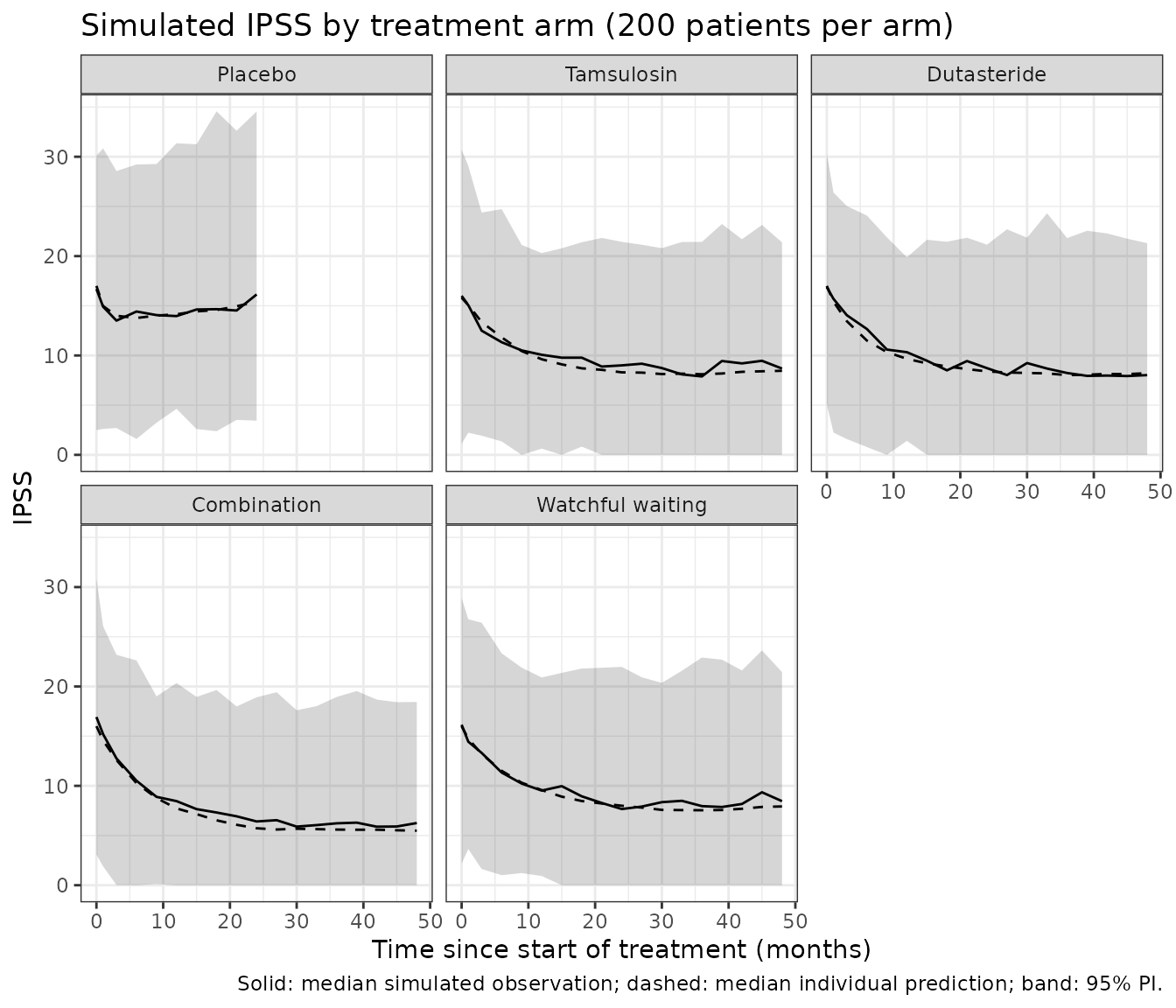
Replicate published figures
Typical-patient trajectories (Figures 5-7)
grid <- tidyr::crossing(IPSS_BL = c(8, 12, 16, 20, 30), arm = arms)
grid$id <- seq_len(nrow(grid))
typ_ev <- do.call(rbind, lapply(seq_len(nrow(grid)), function(i) {
  cbind(
    data.frame(id = grid$id[i], time = 0:48, evid = 0, cmt = "ipss",
               IPSS_BL = grid$IPSS_BL[i], T_SYMPT_BPH = 4, ALCOHOL_USE = 0),
    arm_cov(grid$arm[i])
  )
}))
typ <- as.data.frame(rxode2::rxSolve(mod_typ, typ_ev, returnType = "data.frame"))
#> ℹ omega/sigma items treated as zero: 'etaldisp', 'etaldelta_pbo', 'etalthalf_pbo', 'etaldelta_tamsulosin', 'etaldelta_dutasteride', 'etaldelta_ww', 'etaldelta_fdc'
#> Warning: multi-subject simulation without without 'omega'
typ <- dplyr::select(typ, -dplyr::any_of("IPSS_BL")) |> dplyr::left_join(grid, by = "id")

ggplot(dplyr::filter(typ, arm %in% c("Placebo", "Tamsulosin", "Combination")),
       aes(time, ipss, colour = arm)) +
  geom_line() +
  facet_wrap(~IPSS_BL, labeller = label_both, nrow = 1) +
  labs(x = "Time (months)", y = "IPSS (typical patient)",
       title = "Typical IPSS trajectories by baseline severity (cf. Figures 6 and 7)",
       colour = NULL) +
  theme_bw() + theme(legend.position = "bottom")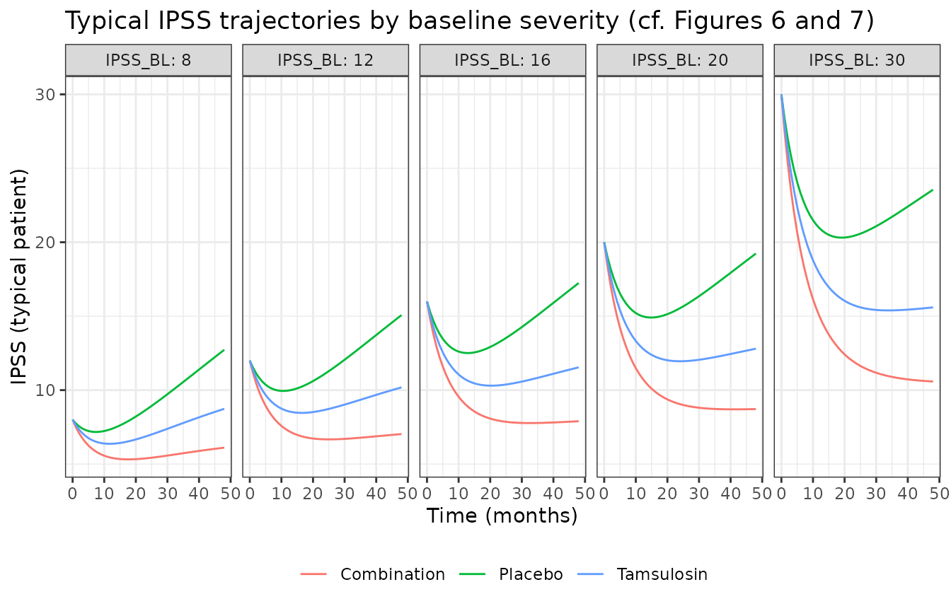
IPSS difference at 48 months versus untreated (Tables S2-S5)
Supporting Information Tables S3 (combination) and S5 (tamsulosin, 50th percentile of DISP) report the median difference at 48 months between the treated and the untreated trajectory. The Table S4 / S5 “moderate” and “severe” columns reproduce the Table S3 IPSSb = 12 and 20 rows exactly (-8.42 and -11.38), so they are taken as baseline IPSS 12 and 20.
d48 <- typ |>
  dplyr::filter(time == 48) |>
  dplyr::select(IPSS_BL, arm, ipss) |>
  tidyr::pivot_wider(names_from = arm, values_from = ipss) |>
  dplyr::mutate(sim_comb = Combination - Placebo, sim_tam = Tamsulosin - Placebo)

pub <- data.frame(
  IPSS_BL = c(8, 12, 16, 20, 30, 12, 20),
  treatment = c(rep("Combination", 5), "Tamsulosin", "Tamsulosin"),
  source = c(rep("Table S3", 5), "Table S5 moderate", "Table S5 severe"),
  published = c(-7.1, -8.42, -10.21, -11.38, -14.41, -5.22, -7.14)
)
cmp <- pub |>
  dplyr::left_join(d48, by = "IPSS_BL") |>
  dplyr::mutate(simulated = ifelse(treatment == "Combination", sim_comb, sim_tam),
                pct_diff = 100 * (simulated / published - 1)) |>
  dplyr::select(source, treatment, IPSS_BL, published, simulated, pct_diff)
cmp |>
  dplyr::rename("Source" = source, "Treatment" = treatment, "Baseline IPSS" = IPSS_BL,
                "Published median" = published, "Typical-value model" = simulated,
                "% difference" = pct_diff) |>
knitr::kable(digits = 2)| Source | Treatment | Baseline IPSS | Published median | Typical-value model | % difference |
|---|---|---|---|---|---|
| Table S3 | Combination | 8 | -7.10 | -6.62 | -6.80 |
| Table S3 | Combination | 12 | -8.42 | -8.05 | -4.43 |
| Table S3 | Combination | 16 | -10.21 | -9.34 | -8.49 |
| Table S3 | Combination | 20 | -11.38 | -10.52 | -7.58 |
| Table S3 | Combination | 30 | -14.41 | -12.97 | -9.99 |
| Table S5 moderate | Tamsulosin | 12 | -5.22 | -4.89 | -6.33 |
| Table S5 severe | Tamsulosin | 20 | -7.14 | -6.43 | -9.88 |
The typical-value model reproduces every published median to within 4-10%, consistently slightly smaller in magnitude. The published values are medians of 200 stochastic simulations whose random-effect settings are not stated (Figure 5 fixes DISP at chosen percentiles and draws the other parameters), whereas the table above uses typical values throughout with a 4-year symptom duration and no alcohol use, so an exact match is not expected. The ordering by baseline severity, the roughly two-fold ratio of combination to tamsulosin benefit, and the magnitudes all agree.
PKNCA validation
Not applicable. The model has no drug concentrations: treatments enter as arm indicators with constant effects, because the source trials collected no pharmacokinetic data (Discussion 4.1). The structural checks above (closed-form steady state and unit conversion) and the Table S2-S5 comparison replace the NCA comparison.
Assumptions and deviations
-
Placebo random-effect block. Table 2 reports only
the variances of the three placebo-model random effects (0.997, 2.822,
2.758). The Supporting Information states that the final model carried
eta correlations between DISP and the placebo magnitude and half-life,
and its control stream fixes an
$OMEGA BLOCK(3)of0.982; -0.977, 3.29; 0.524, -3.01, 2.96, whose diagonal differs slightly from Table 2 (it was most likely carried over from a re-estimation on a different data subset). The model keeps the Table 2 variances and applies the control stream’s correlations (-0.544, 0.307, -0.965) to them. Using the control-stream block verbatim instead changes the variances by at most 17%. -
Arm-dependent random effects. In the authors’
control stream the random effects on DISP and on the placebo magnitude
are applied only to placebo-arm patients (
ARM = 0); in the active arms those two parameters are fixed at their covariate-adjusted typical values, and the between-patient variability is carried by the treatment effect instead (Results 3.3.1). The model reproduces this through the derived indicatorpbo. The placebo half-life keeps its random effect in every arm. -
Covariate functional forms are linear and centred
(
1 + theta (x - ref)), from the control stream. The BMI effects in the control stream are fixed to 0 and are therefore omitted. The control stream sets a factor to 1 when a covariate is missing (-99); supply complete covariates when simulating. - Symptom-duration units. Table 1 reports the duration of BPH symptoms in years (median 4) and the control stream centres it at 4.00, so the coefficient is per year; a Supporting Information table note labels it in months, which is taken as a slip.
-
Supporting Information worked example. The text
illustrating the baseline IPSS effect swaps its two cases: with
DISP x (1 + 0.027 (IPSSb - 16)), IPSSb = 13 gives 0.319 /month and IPSSb = 27 gives 0.450 /month, not the reverse. - Abstract versus tables. The abstract quotes DISP 0.319 /month and treatment effects 0.0139 (tamsulosin) and 0.0310 (combination), which differ from Tables 2 and 3 (0.347, 0.015, 0.032) and match neither the control stream; the tables, which the Results text also quotes, are used.
-
Watchful waiting. CONDUCT’s watchful-waiting arm
(control stream
ARM1 and 2) receives its own constant effect from time 0; the timing of the protocol-defined switch to tamsulosin is not a model input. -
Treatment status before baseline. The control
stream switches all effects off for records with
TREAT = 0(off-treatment records). Time 0 of this model is the start of randomised treatment, and screening observations were excluded from the analysis, so the placebo effect starts at t = 0. - Score bounds. The ODE keeps the score inside (0, 35] on its own, so the control stream’s truncation of the individual prediction is a no-op; its truncation of simulated observations is applied in the simulation above.
- Stochastic versus typical trajectories. The treatment-effect variances (1.4-1.9 on the log scale) are large, and IPSS responds non-linearly to the effect size, so the median simulated trajectory in the active arms runs a few points below the typical-patient curve at 48 months. The paper’s VPCs (Figure 3, Figure S6) were not digitised, so this simulation is not compared against the observed trial data here.
- Residual error is additive with one SD per arm (Tables 2 and 3); the placebo SD was fixed in the final model, the others estimated.