Creatinine with and without a cooked meat meal (Chen 2022)
Source:vignettes/articles/Chen_2022_creatinine.Rmd
Chen_2022_creatinine.RmdModel and source
- Citation: Chen Z, Chen C, Taubert M, Mayersohn M, Fuhr U. A population pharmacokinetic model for creatinine with and without ingestion of a cooked meat meal. Eur J Clin Pharmacol. 2022;78(12):1945-1947. doi:10.1007/s00228-022-03398-9. Data from Mayersohn M, Conrad KA, Achari R. Br J Clin Pharmacol. 1983;15(2):227-230. doi:10.1111/j.1365-2125.1983.tb01490.x.
- Description: One-compartment population pharmacokinetic model for endogenous creatinine in healthy volunteers with and without ingestion of a cooked-beef meal (Chen 2022), a reanalysis of the Mayersohn 1983 plasma and 24 h urine data. Creatinine is generated at a zero-order rate (CGR), eliminated by first-order renal clearance into a cumulative urine state, and the meal creatinine load is absorbed first-order after a lag time. The meal dose is a nominal 180 mg population dose scaled by an estimated dose-correction factor F1. Plasma starts at the endogenous steady state CGR/CL.
- Article: Eur J Clin Pharmacol 2022;78(12):1945-1947 (letter to the editor, open access)
- Original data: Mayersohn et al., Br J Clin Pharmacol 1983;15:227-230
Chen et al. reanalysed the plasma and urine creatinine data of Mayersohn et al. (1983) with a population approach, to estimate the creatinine volume of distribution and generation rate directly rather than fixing the volume to total body water as earlier dynamic creatinine models did. The final model is a single compartment with three fluxes:
- a zero-order endogenous creatinine generation rate (CGR) into plasma,
- first-order renal elimination (CL / Vd), collected in a cumulative urine state,
- first-order absorption, after a lag time, of the creatinine contained in a cooked (boiled) beef meal.
The meal creatinine content was not measured, so the authors gave every subject a nominal population dose of 180 mg and estimated a dose-correction factor F1 (typical value 1.57) with between-subject variability; the individual estimated bioavailable dose was 293 +/- 62.0 mg (n = 6).
Population
The source dataset contains 133 serial creatinine plasma concentrations and 11 creatinine amounts excreted in urine over 24 h from healthy volunteers studied in a control period (no meal) and a beef-ingestion period. The letter states that no demographic information is available in the original publication. The only demographic values it uses are a reference subject of “male, 31 years, 73 kg” (for a Cockcroft-Gault comparison) and a body weight of 73 kg (Vd = 53.9 L is “73.8% of the total body weight”; total body water “43.8 L (60% of 73 kg)”). Six subjects contributed meal-dose estimates (n = 6) and five contributed a beef-period urine collection (n = 5).
The same information is available programmatically via
readModelDb("Chen_2022_creatinine")()$population.
Source trace
Every ini() value carries an in-file comment pointing at
its source. All values are from Table 1 of the letter (final-model
estimates).
| Equation / parameter | Value | Source location |
|---|---|---|
lka |
log(1.76) 1/h | Table 1, Ka |
lcl |
log(7.59) L/h | Table 1, CL (renal clearance) |
lvc |
log(53.9) L | Table 1, Vd |
lfdepot |
log(1.57) | Table 1, F1 (dose correction factor) |
lksyn |
log(67.9) mg/h | Table 1, CGR |
ltlag |
log(0.344) h | Table 1, Lag time |
etalka |
0.26683 | Table 1, IIV Ka 55.3 CV%; log(1 + 0.553^2) |
etalfdepot |
0.058755 | Table 1, IIV F1 24.6 CV%; log(1 + 0.246^2) |
etalksyn |
0.0015199 | Table 1, IIV CGR 3.9 CV%; log(1 + 0.039^2) |
propSd |
0.039 | Table 1, proportional error (plasma) 3.9% |
propSd_Aurine |
0.155 | Table 1, proportional error (urine) 15.5% |
| One compartment, first-order absorption with lag, zero-order generation, linear elimination | n/a | Results, paragraph 1 |
| Exponential IIV; two separate proportional residual errors | n/a | Results, paragraph 1 |
| Population dose 180 mg x individual F1 | n/a | Results, paragraph 1 |
| No IIV on CL or Vd | n/a | Results, paragraph 2 |
central(0) = CGR / CL * Vd (endogenous steady
state) |
n/a | Assumed; see Assumptions and deviations |
Units of every ODE term (time in h, amounts in mg, volumes in L):
| Term | Units | Result |
|---|---|---|
ka * depot |
1/h x mg | mg/h |
ksyn |
mg/h | mg/h |
kel * central = cl / vc * central
|
(L/h / L) x mg | mg/h |
Cc = central / vc |
mg / L | mg/L (Supplementary Fig. 2 axis: mg/L) |
central(0) = ksyn / cl * vc |
(mg/h) / (L/h) x L | mg |
Typical-value checks
mod <- readModelDb("Chen_2022_creatinine")
mod_typ <- mod |> rxode2::zeroRe()
#> ℹ parameter labels from comments will be replaced by 'label()'

ka <- 1.76
cl <- 7.59
vc <- 53.9
fdepot <- 1.57
cgr <- 67.9
tlag <- 0.344
dose_nominal <- 180
kel <- cl / vc
css <- cgr / cl

obs_times <- sort(unique(c(seq(0, 48, by = 0.25), tlag + c(0.01, 0.05, 0.1))))

# Two endpoints (Cc, Aurine): observation rows name an ODE state and carry
# dvid = 1 so rxode2 returns every endpoint column on every row.
obs_rows <- function(times, id = 1L) {
  data.frame(id = id, time = times, evid = 0L, amt = NA_real_, cmt = "central", dvid = 1L)
}
dose_row <- function(id = 1L) {
  data.frame(id = id, time = 0, evid = 1L, amt = dose_nominal, cmt = "depot", dvid = NA_integer_)
}

ev_control <- obs_rows(obs_times)
ev_beef <- rbind(dose_row(), obs_rows(obs_times))

solve_tight <- function(model, ev) {
  out <- rxode2::rxSolve(
    model,
    events = ev, rtol = 1e-10, atol = 1e-12, useLinCmt = FALSE
  ) |>
    as.data.frame()
  if (is.null(out$id)) out$id <- 1L
  out
}

typ_control <- solve_tight(mod_typ, ev_control)
#> ℹ omega/sigma items treated as zero: 'etalka', 'etalfdepot', 'etalksyn'
typ_beef <- solve_tight(mod_typ, ev_beef)
#> ℹ omega/sigma items treated as zero: 'etalka', 'etalfdepot', 'etalksyn'
Steady state without a meal
With no meal, plasma creatinine must stay at CGR / CL = 8.946 mg/L for as long as the solve runs, and the 24 h urinary excretion must equal 24 x CGR = 1629.6 mg (generation balances elimination).
stopifnot(
  max(abs(typ_control$Cc / css - 1)) < 1e-8,
  abs(typ_control$Aurine[typ_control$time == 24] / (24 * cgr) - 1) < 1e-8
)
c(
  Css_model = range(typ_control$Cc),
  Css_expected = css,
  urine24_model = typ_control$Aurine[typ_control$time == 24],
  urine24_expected = 24 * cgr
)
#>       Css_model1       Css_model2     Css_expected    urine24_model
#>         8.945982         8.945982         8.945982      1629.600000
#> urine24_expected
#>      1629.600000
The predicted baseline of 8.95 mg/L matches the flat control-period profile near 9 mg/L in Supplementary Figure 2 of the letter.
Meal profile against the closed form
For a one-compartment model with first-order absorption after a lag and a constant generation rate, the plasma concentration is the steady state plus the standard absorption term:
C(t) = CGR/CL + F1 * D * ka / (Vd * (ka - kel)) * (exp(-kel * (t - tlag)) - exp(-ka * (t - tlag)))
for t > tlag.
closed_form <- function(t) {
  dt <- pmax(t - tlag, 0)
  css + fdepot * dose_nominal * ka / (vc * (ka - kel)) * (exp(-kel * dt) - exp(-ka * dt))
}
rel_err <- abs(typ_beef$Cc / closed_form(typ_beef$time) - 1)
# Both sides use the same parameters, so the difference is pure integration
# error; measured ~5e-11 with rtol = 1e-10.
stopifnot(max(rel_err) < 1e-6)
max(rel_err)
#> [1] 4.667822e-11
Mass balance
All creatinine generated or absorbed must be in the depot, the
plasma, or the urine:
depot + central + urine = central(0) + CGR * t + F1 * D
once the lagged dose has entered the depot.
Derived quantities quoted in the letter
derived <- tibble::tribble(
  ~Quantity, ~Model, ~Paper,
  "Vd as % of 73 kg body weight", 100 * vc / 73, "73.8%",
  "Steady-state plasma creatinine CGR/CL (mg/L)", css, "~9 (Suppl. Fig. 2, control period)",
  "Elimination half-life ln(2) Vd / CL (h)", log(2) * vc / cl, "not reported",
  "Typical bioavailable meal dose F1 x 180 (mg)", fdepot * dose_nominal, "293 +/- 62.0 (individual estimates, n = 6)",
  "Mean bioavailable meal dose, lognormal F1 IIV (mg)",
  fdepot * dose_nominal * exp(0.058755 / 2), "293 +/- 62.0 (individual estimates, n = 6)"
)
stopifnot(abs(100 * vc / 73 - 73.8) < 0.1)
knitr::kable(derived, digits = 2, caption = "Model-implied quantities against the letter's values.")| Quantity | Model | Paper |
|---|---|---|
| Vd as % of 73 kg body weight | 73.84 | 73.8% |
| Steady-state plasma creatinine CGR/CL (mg/L) | 8.95 | ~9 (Suppl. Fig. 2, control period) |
| Elimination half-life ln(2) Vd / CL (h) | 4.92 | not reported |
| Typical bioavailable meal dose F1 x 180 (mg) | 282.60 | 293 +/- 62.0 (individual estimates, n = 6) |
| Mean bioavailable meal dose, lognormal F1 IIV (mg) | 291.03 | 293 +/- 62.0 (individual estimates, n = 6) |
The model-implied mean bioavailable dose (291 mg) agrees with the mean of the six individual estimates the authors report (293 mg).
Virtual cohort and simulation
Supplementary Figure 2 of the letter is a visual predictive check of plasma creatinine over 24 h in the control period and the beef-ingestion period. The cohort below simulates 200 virtual subjects per period with the full model (between-subject variability on Ka, F1 and CGR, plus proportional residual error on the plasma concentrations). No covariates enter the model.
rxode2::rxSetSeed(2022)
n_per_period <- 200L
vpc_times <- c(0, 0.5, 1, 1.5, 2, 3, 4, 5, 6, 7, 8, 10, 12, 15, 18, 21, 24)

make_period <- function(period, id_offset) {
  ids <- id_offset + seq_len(n_per_period)
  obs <- obs_rows(rep(vpc_times, times = length(ids)), id = rep(ids, each = length(vpc_times)))
  dose <- dose_row(ids)
  out <- if (period == "Beef ingestion period") dplyr::bind_rows(dose, obs) else obs
  out |>
    dplyr::mutate(period = period) |>
    dplyr::arrange(id, time, dplyr::desc(evid))
}

events <- dplyr::bind_rows(
  make_period("Control period", 0L),
  make_period("Beef ingestion period", n_per_period)
)
stopifnot(!anyDuplicated(unique(events[, c("id", "time", "evid")])))

sim <- rxode2::rxSolve(mod, events = events, keep = "period", useLinCmt = FALSE) |>
  as.data.frame() |>
  dplyr::mutate(period = factor(period, levels = c("Control period", "Beef ingestion period")))
#> ℹ parameter labels from comments will be replaced by 'label()'
stopifnot(!anyNA(sim$Cc))

# `Cc` in the solve output is the individual prediction; add the plasma
# proportional residual error (3.9%) explicitly for the VPC.
set.seed(2022)
sim$Cc_obs <- sim$Cc * (1 + 0.039 * stats::rnorm(nrow(sim)))
Supplementary Figure 2
# Replicates Supplementary Figure 2 of Chen 2022: VPC of plasma creatinine,
# control period and beef-ingestion period.
vpc <- sim |>
  dplyr::group_by(period, time) |>
  dplyr::summarise(
    Q05 = quantile(Cc_obs, 0.05),
    Q50 = quantile(Cc_obs, 0.50),
    Q95 = quantile(Cc_obs, 0.95),
    .groups = "drop"
  )

ggplot(vpc, aes(time, Q50)) +
  geom_ribbon(aes(ymin = Q05, ymax = Q95), alpha = 0.25, fill = "steelblue") +
  geom_line() +
  facet_wrap(~period) +
  labs(
    x = "Time (h)",
    y = "Creatinine plasma concentration (mg/L)",
    title = "Simulated 5th, 50th and 95th percentiles",
    caption = "Replicates Supplementary Figure 2 of Chen 2022 (200 virtual subjects per period)."
  )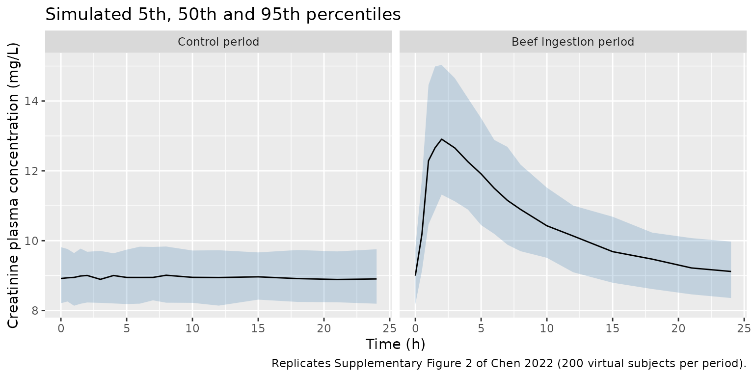
The simulated control period is flat near 9 mg/L and the beef-ingestion median peaks at about 13 mg/L between 1 and 3 h after the meal, falling back towards baseline by 24 h. The observed medians in Supplementary Figure 2 behave the same way: about 9 mg/L throughout the control period, and in the beef period a peak of about 12.5-13 mg/L between 1 and 5 h, about 10 mg/L at 12 h and about 9.6 mg/L at 18-24 h.
med <- function(p, t) vpc$Q50[vpc$period == p & vpc$time == t]
stopifnot(
  # Control period: the centre sits at CGR/CL; a 10% band admits sampling noise
  # (CGR IIV is 3.9% and residual error 3.9%) and still breaks on a wrong CL or CGR.
  abs(med("Control period", 12) / css - 1) < 0.10,
  # Beef period: median at 2 h is about 13 mg/L and returns within 15% of baseline by 24 h.
  med("Beef ingestion period", 2) > 11.5,
  med("Beef ingestion period", 2) < 15,
  abs(med("Beef ingestion period", 24) / css - 1) < 0.15
)
PKNCA validation
The letter reports no NCA. PKNCA is used here on the meal-derived
excess concentration (plasma creatinine minus each subject’s own
endogenous steady state ksyn / cl), for which
AUC0-inf = F1 * D / CL and the terminal half-life is
ln(2) * Vd / CL exactly. The typical-value subject gives a
deterministic check; the cohort gives the distribution.
nca_times <- c(0, 0.25, 0.5, 0.75, 1, 1.25, 1.5, 2, 2.5, 3, 4, 5, 6, 8, 10, 12, 16, 20, 24, 30, 36, 48, 60, 72)

ev_nca <- dplyr::bind_rows(
  dose_row(1:200),
  obs_rows(rep(nca_times, times = 200), id = rep(1:200, each = length(nca_times)))
) |>
  dplyr::mutate(treatment = "Beef meal, 180 mg nominal") |>
  dplyr::arrange(id, time, dplyr::desc(evid))

sim_nca <- rxode2::rxSolve(mod, events = ev_nca, keep = "treatment", useLinCmt = FALSE) |>
  as.data.frame() |>
  dplyr::mutate(Cc = Cc - ksyn / cl)

typ_nca <- rxode2::rxSolve(
  mod_typ,
  events = ev_nca |> dplyr::filter(id == 1),
  rtol = 1e-10, atol = 1e-12, useLinCmt = FALSE,
  keep = "treatment"
) |>
  as.data.frame() |>
  dplyr::mutate(id = 1L, Cc = Cc - ksyn / cl, treatment = "Typical value")
#> ℹ omega/sigma items treated as zero: 'etalka', 'etalfdepot', 'etalksyn'

run_nca <- function(conc_df, dose_df) {
  # Integration noise around zero at time 0 and in the far tail is floored.
  stopifnot(all(conc_df$Cc >= -1e-6 * max(conc_df$Cc)))
  conc <- conc_df |>
    dplyr::filter(!is.na(Cc)) |>
    dplyr::mutate(Cc = pmax(Cc, 0)) |>
    dplyr::select(id, time, Cc, treatment)
  conc_obj <- PKNCA::PKNCAconc(conc, Cc ~ time | treatment + id)
  dose_obj <- PKNCA::PKNCAdose(dose_df, amt ~ time | treatment + id)
  intervals <- data.frame(
    start = 0, end = Inf,
    cmax = TRUE, tmax = TRUE, aucinf.obs = TRUE, half.life = TRUE
  )
  PKNCA::pk.nca(PKNCA::PKNCAdata(conc_obj, dose_obj, intervals = intervals))
}

dose_cohort <- ev_nca |>
  dplyr::filter(evid == 1) |>
  dplyr::select(id, time, amt, treatment)
nca_cohort <- run_nca(sim_nca, dose_cohort)
nca_typ <- run_nca(
  typ_nca,
  dose_cohort |> dplyr::filter(id == 1) |> dplyr::mutate(treatment = "Typical value")
)

res <- dplyr::bind_rows(as.data.frame(nca_typ), as.data.frame(nca_cohort)) |>
  dplyr::filter(PPTESTCD %in% c("cmax", "tmax", "aucinf.obs", "half.life")) |>
  dplyr::group_by(treatment, PPTESTCD) |>
  dplyr::summarise(median = median(PPORRES), .groups = "drop") |>
  tidyr::pivot_wider(names_from = PPTESTCD, values_from = median)

auc_expected <- fdepot * dose_nominal / cl
thalf_expected <- log(2) * vc / cl
tmax_expected <- tlag + log(ka / kel) / (ka - kel)
cmax_expected <- closed_form(tmax_expected) - css

typ_row <- res[res$treatment == "Typical value", ]
coh_row <- res[res$treatment != "Typical value", ]
stopifnot(
  # Typical value: trapezoidal error on the sampling grid only.
  abs(typ_row$aucinf.obs / auc_expected - 1) < 0.02,
  abs(typ_row$half.life / thalf_expected - 1) < 0.01,
  abs(typ_row$cmax / cmax_expected - 1) < 0.02,
  # Cohort: AUC depends only on F1 (24.6% CV), so its median sits at the
  # typical value; the sampling SE of a 200-subject median is about 2%.
  abs(coh_row$aucinf.obs / auc_expected - 1) < 0.10
)

res |>
  dplyr::bind_rows(tibble::tibble(
    treatment = "Closed form (typical)",
    cmax = cmax_expected, tmax = tmax_expected,
    aucinf.obs = auc_expected, half.life = thalf_expected
  )) |>
  dplyr::rename(
    "Group" = treatment,
    "Excess Cmax (mg/L)" = cmax,
    "Tmax (h)" = tmax,
    "Excess AUC0-inf (mg*h/L)" = aucinf.obs,
    "t1/2 (h)" = half.life
  ) |>
  knitr::kable(
    digits = 3,
    caption = "PKNCA on the meal-derived excess plasma creatinine (median for the cohort)."
)| Group | Excess AUC0-inf (mg*h/L) | Excess Cmax (mg/L) | t1/2 (h) | Tmax (h) |
|---|---|---|---|---|
| Beef meal, 180 mg nominal | 35.657 | 3.979 | 4.930 | 2.000 |
| Typical value | 37.225 | 4.205 | 4.927 | 2.000 |
| Closed form (typical) | 37.233 | 4.209 | 4.922 | 1.904 |
Urinary excretion
The model predicts the 24 h urinary creatinine excretion as the endogenous generation over 24 h plus the fraction of the absorbed meal creatinine eliminated by 24 h.
urine24 <- tibble::tibble(
  Period = c("Control", "Beef ingestion"),
  `Typical 24 h urine creatinine (mg)` = c(
    typ_control$Aurine[typ_control$time == 24],
    typ_beef$Aurine[typ_beef$time == 24]
  )
) |>
  dplyr::mutate(`Excess over control (mg)` = `Typical 24 h urine creatinine (mg)` -
    `Typical 24 h urine creatinine (mg)`[1])
knitr::kable(urine24, digits = 1)| Period | Typical 24 h urine creatinine (mg) | Excess over control (mg) |
|---|---|---|
| Control | 1629.6 | 0.0 |
| Beef ingestion | 1901.2 | 271.6 |
The predicted excess of about 272 mg is the typical bioavailable dose eliminated within 24 h. The letter itself notes that the individual estimated doses (293 +/- 62.0 mg, n = 6) were “not fully consistent with the increased creatinine amount excreted in urine after beef ingestion (180 +/- 102 mg, n = 5)” and attributes the gap possibly to the accuracy of the raw data; the packaged model reproduces the authors’ fitted parameters, not that raw urine difference.
Assumptions and deviations
- CL value. Table 1 gives CL = 7.59 L/h and the Results prose quotes “7.92 L/h”. The table value is used: its bootstrap median (7.59) and 95% CI (6.71-8.48) are centred on it, and CGR / CL = 67.9 / 7.59 = 8.95 mg/L reproduces the control-period level near 9 mg/L in Supplementary Figure 2, whereas 67.9 / 7.92 = 8.57 mg/L would sit below it. Likewise the prose quotes CGR as 68.0 mg/h against 67.9 mg/h in Table 1; the table value is used.
-
IIV scale. Table 1 reports the between-subject
variability only as CV%. With exponential IIV, the variances are
computed as
log(1 + CV^2); for the CVs reported (55.3%, 24.6%, 3.9%) the alternativeCV^2reading would give 0.306, 0.0605 and 0.00152. -
Initial condition. The letter does not state how
the pre-meal baseline was handled. Plasma creatinine is initialised at
the endogenous steady state
CGR / CL, which is what a constant generation rate with first-order elimination implies and what the flat control-period VPC shows. -
Meal dose. The model reproduces the authors’
parameterisation: dose the nominal 180 mg into
depotand the estimated F1 (1.57) scales it to the bioavailable amount. Dosing a measured meal creatinine content instead would over-predict the absorbed amount by the factor F1. -
Urine collection. The 24 h urine amounts are
modelled as the cumulative
urinestate from time 0; the start of the collection is assumed to coincide with the meal. - Population. The original study’s demographics are not available; the number of subjects (6) is inferred from the “n = 6” individual dose estimates. No covariates enter the model.
- Errata. No correction notice was found for the letter as of 2026-10-10.