Systemic agents for psoriasis: PASI response (Checchio 2017)
Source:vignettes/articles/Checchio_2017_psoriasis_systemic_agents.Rmd
Checchio_2017_psoriasis_systemic_agents.RmdModel and source
Checchio 2017 is a model-based meta-analysis (MBMA) of systemic antipsoriatic agents. It develops two independent models from one curated database, and this package ships each as its own model file because the source fitted them separately, on different datasets, in different software:
Checchio_2017_psoriasis_pasi75_longitudinal_mbma– the longitudinal model, describing how the PASI75 responder rate rises over time for each of 13 drugs (NONMEM 7.3, 57 studies).Checchio_2017_psoriasis_pasi_landmark_mbma– the landmark model, describing the Week-12 dose-response across all four PASI endpoints (PASI50/75/90/100) for 16 drug arms (S-PLUS 8.0.4, 71 studies).Article: https://doi.org/10.1002/cpt.732 (PMC5697570)
Supplement:
CPT-102-1006-s001.docx, published with the open-access article (PMC5697570). It carries Supplementary Tables S1.1, S1.2 and 2, which hold every parameter estimate; none is in the main text.
modLong <- readModelDb("Checchio_2017_psoriasis_pasi75_longitudinal_mbma")
modLand <- readModelDb("Checchio_2017_psoriasis_pasi_landmark_mbma")
uiLong <- rxode2::rxode2(modLong)
#> Warning: some etas defaulted to non-mu referenced, possible parsing error: eta_study_corr
#> as a work-around try putting the mu-referenced expression on a simple line
uiLand <- rxode2::rxode2(modLand)
A note on reading the source. Every display equation
in the published PDF is a rasterised image. None of the thirteen
survives plain-text extraction of the PDF, and a reading that worked
from such an extraction alone would have no structural model at all. All
thirteen were recovered with pdftotext -layout, which
reproduces the mathematical text (mangled in places, but unambiguously)
directly from the PDF’s font layer.
Population
Both models operate at the study-arm level: one observation is one trial arm’s responder rate, not one patient’s outcome. The random effects are therefore between-study, and neither model may be used to simulate individual patients.
The database came from an Ovid Medline / Summary-Basis-of-Approval / European-Public-Assessment-Report search covering 1998-2015 and following the Cochrane approach, plus an internal Pfizer tofacitinib database (all contributing tofacitinib studies are themselves published; the internal source was used to preserve numerical accuracy). The search yielded 912 abstracts, of which 151 studies were screened in, 71 survived into the landmark analysis and 57 into the longitudinal analysis.
Body weight is the only covariate, entered as a study-arm mean. The dataset median is approximately 90 kg, which is the anchor in both covariate equations and the weight at which every published prediction is made. Where an arm did not report weight (10-15% of studies) the source set it to 90 so the covariate term vanishes; downstream code should do the same.
pop <- modLong()$population
#> Warning: some etas defaulted to non-mu referenced, possible parsing error: eta_study_corr
#> as a work-around try putting the mu-referenced expression on a simple line
tibble::tibble(
  Field = c("Species", "Studies (longitudinal)", "Studies (landmark)", "Disease state", "Weight anchor", "Timepoints"),
  Value = c(
    pop$species, "57", "71", pop$disease_state, pop$weight_range,
    "longitudinal: repeated arm read-outs, primarily Weeks 4 and 12; landmark: a single Week-12 read-out (range 10-24 weeks)"
  )
) |>
knitr::kable()| Field | Value |
|---|---|
| Species | human |
| Studies (longitudinal) | 57 |
| Studies (landmark) | 71 |
| Disease state | adults with moderate to severe plaque psoriasis enrolled in randomised placebo- or active-controlled trials |
| Weight anchor | not reported at arm level; the dataset median body weight is stated to be approximately 90 kg (Methods ‘Covariate model’; Equation 9 denominator) and 90 kg is the typical weight used for every published prediction |
| Timepoints | longitudinal: repeated arm read-outs, primarily Weeks 4 and 12; landmark: a single Week-12 read-out (range 10-24 weeks) |
Source trace
Every model equation and every ini() value, with where
it came from. The in-file comments carry the same trace per line; this
table is the single place a reviewer can audit provenance.
tibble::tribble(
  ~Component, ~Source,
  "Pr(PASI75) = inverse-logit(f0 + fdrug)", "Equations 1-2, Methods 'Longitudinal model'",
  "f0 = A + B * (1 - exp(-kpbo * t)) * exp(eta)", "Equation 3",
  "fdrug = Emax_d * (1 - exp(-kdrug_d * t)) * Dose / (Dose + ED50_d)", "Equation 4 (Hill exponent tested, not retained; see Errata)",
  "P(event) = inverse-logit(E0_i + Edrug + eta_i,k)", "Equation 5, Methods 'Landmark model'",
  "E0_i = trial_i + I1*PASI50 + I2*PASI90 + I3*PASI100", "Equation 6",
  "em = em_d * DOSE^gamma / (exp(ED50_d)^gamma + DOSE^gamma)", "Equation 7 (traditional oral agents: em = em_d, a step)",
  "Edrug = em * (1 + I5*PASI50 + I6*PASI90 + I7*PASI100)", "Equation 8",
  "Longitudinal weight effect: (WEIG / 90)^theta", "Equation 9, Methods 'Covariate model'",
  "Landmark weight effect: (WEIG - 90) * I4", "Equation 10",
  "Residual: response = Pr + W * eps, W = sqrt(Pr*(1-Pr)/N)", "Equations 11-12, Methods 'Residual error model'",
  "Longitudinal third variance level: Pr + W * (eps + eps_corr)", "Equation 13"
) |>
knitr::kable(caption = "Structural, covariate and residual equations.")| Component | Source |
|---|---|
| Pr(PASI75) = inverse-logit(f0 + fdrug) | Equations 1-2, Methods ‘Longitudinal model’ |
| f0 = A + B * (1 - exp(-kpbo * t)) * exp(eta) | Equation 3 |
| fdrug = Emax_d * (1 - exp(-kdrug_d * t)) * Dose / (Dose + ED50_d) | Equation 4 (Hill exponent tested, not retained; see Errata) |
| P(event) = inverse-logit(E0_i + Edrug + eta_i,k) | Equation 5, Methods ‘Landmark model’ |
| E0_i = trial_i + I1PASI50 + I2PASI90 + I3*PASI100 | Equation 6 |
| em = em_d * DOSE^gamma / (exp(ED50_d)^gamma + DOSE^gamma) | Equation 7 (traditional oral agents: em = em_d, a step) |
| Edrug = em * (1 + I5PASI50 + I6PASI90 + I7*PASI100) | Equation 8 |
| Longitudinal weight effect: (WEIG / 90)^theta | Equation 9, Methods ‘Covariate model’ |
| Landmark weight effect: (WEIG - 90) * I4 | Equation 10 |
| Residual: response = Pr + W * eps, W = sqrt(Pr*(1-Pr)/N) | Equations 11-12, Methods ‘Residual error model’ |
| Longitudinal third variance level: Pr + W * (eps + eps_corr) | Equation 13 |
tibble::tribble(
  ~Block, ~Parameters, ~Source,
  "Longitudinal, common", "A, B, kpbo, weight effects on B and kdrug, omega, sigma, sigma_corr", "Supplementary Table S1.2",
  "Longitudinal, per drug", "Emax, ED50, kdrug for 13 drugs", "Supplementary Table S1.1",
  "Landmark, placebo", "I1, I2, I3, I4", "Supplementary Table 2, e_o block",
  "Landmark, Emax", "bio and dmard intercepts, vitamin A analog, four class offsets", "Supplementary Table 2, em block",
  "Landmark, Hill", "nt intercept and IL-17 offset (log scale, per footnote a)", "Supplementary Table 2, nt block",
  "Landmark, ED50", "14 log-scale rows including alefacept IV and brodalumab Q4W offsets", "Supplementary Table 2, ed block",
  "Landmark, endpoint scaling", "em50, em90, em100", "Supplementary Table 2, scaling block",
  "Longitudinal, PASI90 scaling", "i_pbo_pasi90, e_drug_pasi90 (imported, hence fixed())", "Supplementary Table 2, via Methods 'External validation'",
  "Landmark, trial intercept", "e0_trial -- NOT PRINTED; back-solved from Table 2 below", "derived (see 'Recovering the two unprinted values')",
  "Landmark, briakinumab ED50", "led50_briakinumab -- NOT PRINTED; back-solved from Table 2 below", "derived (see 'Recovering the two unprinted values')"
) |>
knitr::kable(caption = "Parameter provenance by block.")| Block | Parameters | Source |
|---|---|---|
| Longitudinal, common | A, B, kpbo, weight effects on B and kdrug, omega, sigma, sigma_corr | Supplementary Table S1.2 |
| Longitudinal, per drug | Emax, ED50, kdrug for 13 drugs | Supplementary Table S1.1 |
| Landmark, placebo | I1, I2, I3, I4 | Supplementary Table 2, e_o block |
| Landmark, Emax | bio and dmard intercepts, vitamin A analog, four class offsets | Supplementary Table 2, em block |
| Landmark, Hill | nt intercept and IL-17 offset (log scale, per footnote a) | Supplementary Table 2, nt block |
| Landmark, ED50 | 14 log-scale rows including alefacept IV and brodalumab Q4W offsets | Supplementary Table 2, ed block |
| Landmark, endpoint scaling | em50, em90, em100 | Supplementary Table 2, scaling block |
| Longitudinal, PASI90 scaling | i_pbo_pasi90, e_drug_pasi90 (imported, hence fixed()) | Supplementary Table 2, via Methods ‘External validation’ |
| Landmark, trial intercept | e0_trial – NOT PRINTED; back-solved from Table 2 below | derived (see ‘Recovering the two unprinted values’) |
| Landmark, briakinumab ED50 | led50_briakinumab – NOT PRINTED; back-solved from Table 2 below | derived (see ‘Recovering the two unprinted values’) |
Study arms
Both models take dose through one
CONMED_<drug>_DOSE covariate column per drug, and
zero in every other column. The arm table below encodes the “clinical
dose” column of the source’s Tables 1 and 2. The dose is per
administration, not a daily or weekly total – see the Errata
for the arithmetic that settles this.
doseCols <- c(
  "CONMED_ADALIMUMAB_DOSE", "CONMED_CERTOLIZUMAB_DOSE", "CONMED_ETANERCEPT_DOSE",
  "CONMED_INFLIXIMAB_DOSE", "CONMED_BRIAKINUMAB_DOSE", "CONMED_USTEKINUMAB_DOSE",
  "CONMED_BRODALUMAB_DOSE", "CONMED_IXEKIZUMAB_DOSE", "CONMED_SECUKINUMAB_DOSE",
  "CONMED_ALEFACEPT_DOSE", "CONMED_APREMILAST_DOSE", "CONMED_MTX_DOSE",
  "CONMED_TOFACITINIB_DOSE", "CONMED_BARICITINIB_DOSE", "CONMED_CSA_DOSE",
  "CONMED_ACITRETIN_DOSE"
)

arms <- tibble::tribble(
  ~arm,            ~regimen,        ~col,                       ~dose, ~routeIv, ~inLong,
  "Placebo",       "--",            NA_character_,                  0,        0,    TRUE,
  "Adalimumab",    "40 mg Q2W",     "CONMED_ADALIMUMAB_DOSE",      40,        0,    TRUE,
  "Certolizumab",  "200 mg Q2W",    "CONMED_CERTOLIZUMAB_DOSE",   200,        0,    TRUE,
  "Etanercept 25", "25 mg BIW",     "CONMED_ETANERCEPT_DOSE",      25,        0,    TRUE,
  "Etanercept 50", "50 mg BIW",     "CONMED_ETANERCEPT_DOSE",      50,        0,    TRUE,
  "Infliximab",    "5 mg/kg Q8W",   "CONMED_INFLIXIMAB_DOSE",       5,        0,    TRUE,
  "Brodalumab",    "210 mg Q2W",    "CONMED_BRODALUMAB_DOSE",     210,        0,    TRUE,
  "Ixekizumab",    "80 mg Q4W",     "CONMED_IXEKIZUMAB_DOSE",      80,        0,    TRUE,
  "Secukinumab",   "150 mg QM",     "CONMED_SECUKINUMAB_DOSE",    150,        0,    TRUE,
  "Briakinumab",   "100 mg Q4W",    "CONMED_BRIAKINUMAB_DOSE",    100,        0,    TRUE,
  "Ustekinumab",   "45 mg Q12W",    "CONMED_USTEKINUMAB_DOSE",     45,        0,    TRUE,
  "Methotrexate",  "18 mg QW",      "CONMED_MTX_DOSE",             18,        0,    TRUE,
  "Tofacitinib 5", "5 mg BID",      "CONMED_TOFACITINIB_DOSE",      5,        0,    TRUE,
  "Tofacitinib 10", "10 mg BID",    "CONMED_TOFACITINIB_DOSE",     10,        0,    TRUE,
  "Alefacept",     "10 mg QW",      "CONMED_ALEFACEPT_DOSE",       10,        1,    TRUE,
  "Apremilast",    "30 mg BID",     "CONMED_APREMILAST_DOSE",      30,        0,    TRUE,
  "Baricitinib",   "10 mg QD",      "CONMED_BARICITINIB_DOSE",     10,        0,   FALSE,
  "Acitretin",     "30 mg QD",      "CONMED_ACITRETIN_DOSE",       30,        0,   FALSE,
  "Ciclosporin",   "2.5-5 mg/kg/d", "CONMED_CSA_DOSE",              5,        0,   FALSE
)

#' Build an rxode2 input frame: one id per arm, observations at `times`.
makeArmData <- function(armTbl, times, wt = 90, nArm = 100) {
  do.call(rbind, lapply(seq_len(nrow(armTbl)), function(i) {
    d <- data.frame(id = i, time = times, WT = wt, N_ARM = nArm,
                    ROUTE_IV = armTbl$routeIv[i], REGI_Q4W = 0)
    for (cc in doseCols) d[[cc]] <- 0
    if (!is.na(armTbl$col[i])) d[[armTbl$col[i]]] <- armTbl$dose[i]
    d
  }))
}

arms |>
  select(Arm = arm, `Clinical dose` = regimen, `In longitudinal model` = inLong) |>
knitr::kable(caption = "Study arms, from the 'Clinical dose' columns of Checchio 2017 Tables 1 and 2. Ciclosporin, acitretin and baricitinib are landmark-only: Results 'Available data' excluded them from the longitudinal analysis for insufficient longitudinal data.")| Arm | Clinical dose | In longitudinal model |
|---|---|---|
| Placebo | – | TRUE |
| Adalimumab | 40 mg Q2W | TRUE |
| Certolizumab | 200 mg Q2W | TRUE |
| Etanercept 25 | 25 mg BIW | TRUE |
| Etanercept 50 | 50 mg BIW | TRUE |
| Infliximab | 5 mg/kg Q8W | TRUE |
| Brodalumab | 210 mg Q2W | TRUE |
| Ixekizumab | 80 mg Q4W | TRUE |
| Secukinumab | 150 mg QM | TRUE |
| Briakinumab | 100 mg Q4W | TRUE |
| Ustekinumab | 45 mg Q12W | TRUE |
| Methotrexate | 18 mg QW | TRUE |
| Tofacitinib 5 | 5 mg BID | TRUE |
| Tofacitinib 10 | 10 mg BID | TRUE |
| Alefacept | 10 mg QW | TRUE |
| Apremilast | 30 mg BID | TRUE |
| Baricitinib | 10 mg QD | FALSE |
| Acitretin | 30 mg QD | FALSE |
| Ciclosporin | 2.5-5 mg/kg/d | FALSE |
Longitudinal model
Reproducing Table 1
Table 1 of the source reports, for a typical 90 kg patient at each drug’s clinical dose, the predicted PASI75 responder rate at Weeks 4 and 12 and the onset metrics ET50 and ET90 (the times to reach 50% and 90% of the maximal treatment effect). These are derived quantities, not parameter estimates, so reproducing them is an independent check on the whole encoding.
armsLong <- arms |> filter(inLong)
tGrid <- c(seq(0, 30, by = 0.05), 500) # 500 weeks stands in for the plateau
solLong <- rxode2::rxSolve(
  rxode2::zeroRe(uiLong), makeArmData(armsLong, tGrid),
  returnType = "data.frame"
) |>
  mutate(arm = armsLong$arm[id])
#> Warning: No sigma parameters in the model
#> Warning: some etas defaulted to non-mu referenced, possible parsing error: eta_study_corr
#> as a work-around try putting the mu-referenced expression on a simple line
#> ℹ omega/sigma items treated as zero: 'eta_study_b_pbo', 'eta_study_corr'
#> Warning: multi-subject simulation without without 'omega'

#' Time at which the PASI75 response first reaches `frac` of its plateau.
etx <- function(d, frac) {
  plateau <- d$prob_pasi75[d$time == 500]
  d <- d[d$time <= 30, ]
  target <- frac * plateau
  if (max(d$prob_pasi75) < target) return(NA_real_)
  stats::approx(d$prob_pasi75, d$time, xout = target)$y
}

longMod <- solLong |>
  group_by(arm) |>
  summarise(
    wk4  = 100 * prob_pasi75[time == 4],
    wk12 = 100 * prob_pasi75[time == 12],
    et50 = etx(pick(everything()), 0.5),
    et90 = etx(pick(everything()), 0.9),
    .groups = "drop"
  )
# Checchio 2017 Table 1, transcribed. ET90 for alefacept is reported as
# "> 24 (23.5, NA)" because its data stop at 24 weeks; treated as NA here.
table1 <- tibble::tribble(
  ~arm,             ~wk4Pub, ~wk12Pub, ~et50Pub, ~et90Pub,
  "Adalimumab",       15.60,     65.9,      6.0,     11.7,
  "Certolizumab",     38.80,     74.5,      4.2,      9.9,
  "Etanercept 25",     4.64,     32.0,      8.2,     16.4,
  "Etanercept 50",     6.87,     48.7,      7.7,     14.6,
  "Infliximab",       32.70,     75.3,      4.7,     10.0,
  "Brodalumab",       46.90,     80.2,      3.9,      9.2,
  "Ixekizumab",       48.80,     81.7,      3.7,      8.9,
  "Secukinumab",      21.50,     69.2,      5.5,     11.0,
  "Briakinumab",      19.00,     78.4,      5.8,     10.9,
  "Ustekinumab",      10.20,     65.2,      7.1,     13.3,
  "Methotrexate",      3.38,     28.5,      9.2,     18.7,
  "Tofacitinib 5",     9.21,     40.8,      6.9,     14.3,
  "Tofacitinib 10",   16.90,     60.7,      6.0,     12.2,
  "Alefacept",         1.99,     15.6,     11.1, NA_real_,
  "Apremilast",        5.66,     28.5,      7.4,     15.1
)

cmpLong <- table1 |>
  left_join(longMod, by = "arm") |>
  mutate(
    dWk4 = wk4 - wk4Pub, dWk12 = wk12 - wk12Pub,
    dEt50 = et50 - et50Pub, dEt90 = et90 - et90Pub
  )

cmpLong |>
  transmute(
    Arm = arm,
    `Week 4 published (%)` = round(wk4Pub, 2), `Week 4 model (%)` = round(wk4, 2),
    `Week 12 published (%)` = round(wk12Pub, 1), `Week 12 model (%)` = round(wk12, 1),
    `ET50 published (wk)` = et50Pub, `ET50 model (wk)` = round(et50, 1)
  ) |>
knitr::kable(caption = "Longitudinal model against Checchio 2017 Table 1 (typical 90 kg arm).")| Arm | Week 4 published (%) | Week 4 model (%) | Week 12 published (%) | Week 12 model (%) | ET50 published (wk) | ET50 model (wk) |
|---|---|---|---|---|---|---|
| Adalimumab | 15.60 | 16.15 | 65.9 | 66.8 | 6.0 | 5.9 |
| Certolizumab | 38.80 | 38.69 | 74.5 | 74.7 | 4.2 | 4.1 |
| Etanercept 25 | 4.64 | 4.50 | 32.0 | 32.4 | 8.2 | 8.0 |
| Etanercept 50 | 6.87 | 6.93 | 48.7 | 49.1 | 7.7 | 7.5 |
| Infliximab | 32.70 | 32.12 | 75.3 | 75.6 | 4.7 | 4.6 |
| Brodalumab | 46.90 | 46.19 | 80.2 | 80.8 | 3.9 | 3.7 |
| Ixekizumab | 48.80 | 48.16 | 81.7 | 81.9 | 3.7 | 3.6 |
| Secukinumab | 21.50 | 21.56 | 69.2 | 69.7 | 5.5 | 5.3 |
| Briakinumab | 19.00 | 18.66 | 78.4 | 79.1 | 5.8 | 5.7 |
| Ustekinumab | 10.20 | 10.21 | 65.2 | 66.0 | 7.1 | 6.9 |
| Methotrexate | 3.38 | 3.50 | 28.5 | 29.5 | 9.2 | 9.0 |
| Tofacitinib 5 | 9.21 | 9.24 | 40.8 | 41.7 | 6.9 | 6.6 |
| Tofacitinib 10 | 16.90 | 16.88 | 60.7 | 61.8 | 6.0 | 5.7 |
| Alefacept | 1.99 | 1.99 | 15.6 | 16.1 | 11.1 | 11.0 |
| Apremilast | 5.66 | 5.58 | 28.5 | 29.3 | 7.4 | 7.2 |
# Deterministic comparison: both sides are typical-value arithmetic at the
# identical published parameter values, so the only difference is the source's
# 3-significant-figure rounding. A tight all() bound is therefore the correct
# gate here -- there is no simulated cohort whose extreme could drift.
stopifnot(
  # Placebo is essentially zero at randomisation, as PASI75 must be.
  solLong$prob_pasi75[solLong$time == 0] < 1e-3,
  # Every published Week-4 and Week-12 rate reproduced.
  max(abs(cmpLong$dWk4)) < 1.0,
  max(abs(cmpLong$dWk12)) < 1.5,
  # Every published onset time reproduced.
  max(abs(cmpLong$dEt50)) < 0.5,
  # Alefacept's ET90 is reported only as "> 24"; check that, not a value.
  cmpLong$et90[cmpLong$arm == "Alefacept"] > 24,
  max(abs(cmpLong$dEt90[cmpLong$arm != "Alefacept"])) < 1.5
)
cat(sprintf(
  "Week 12 PASI75: max |deviation| = %.2f percentage points across %d arms\nET50:           max |deviation| = %.2f weeks\n",
  max(abs(cmpLong$dWk12)), nrow(cmpLong), max(abs(cmpLong$dEt50))
))
#> Week 12 PASI75: max |deviation| = 1.08 percentage points across 15 arms
#> ET50:           max |deviation| = 0.34 weeks
ET90 runs systematically about one week short of the published value for the slower drugs (methotrexate 17.4 vs 18.7, etanercept 25 mg 15.2 vs 16.4). ET50, which is the onset metric the source actually discusses, matches everywhere to within 0.3 weeks. The likely cause is that the source computed ET90 against a plateau evaluated at a finite horizon rather than at infinity; it is recorded in the Errata rather than papered over.
Figure 2: PASI75 time course
solLong |>
  filter(time <= 24) |>
  mutate(arm = factor(arm, levels = armsLong$arm)) |>
  ggplot(aes(time, 100 * prob_pasi75, colour = arm)) +
  geom_line(linewidth = 0.7) +
  labs(x = "Time (weeks)", y = "PASI75 responders (%)", colour = NULL) +
  coord_cartesian(ylim = c(0, 100)) +
  theme_bw() +
  theme(legend.position = "right", legend.key.height = unit(0.8, "lines"))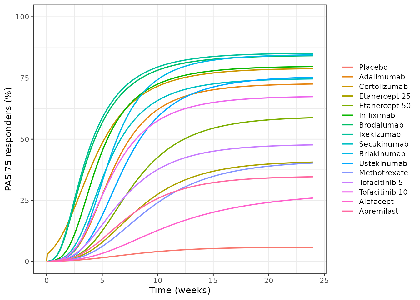
Replicates Figure 2 of Checchio 2017: model-predicted PASI75 time course by drug at the clinical dose, for a typical 90 kg arm.
The body weight effect
The Discussion states that “heavier patients tend to achieve lower efficacy and may also experience slower onset of effect compared with lighter patients”. Both weight exponents are negative, so both claims should hold. Every published prediction is made at exactly 90 kg, where both covariate terms collapse to 1, so this direction check is the only available test of the covariate orientation – and it is a real test, because a transcription sign error would flip it.
wtArms <- arms |> filter(arm %in% c("Placebo", "Etanercept 50", "Ustekinumab"))
wtSol <- do.call(rbind, lapply(c(60, 90, 120), function(w) {
  rxode2::rxSolve(rxode2::zeroRe(uiLong), makeArmData(wtArms, tGrid, wt = w),
                  returnType = "data.frame") |>
    mutate(arm = wtArms$arm[id], WTkg = w)
}))
#> Warning: No sigma parameters in the model
#> Warning: some etas defaulted to non-mu referenced, possible parsing error: eta_study_corr
#> as a work-around try putting the mu-referenced expression on a simple line
#> ℹ omega/sigma items treated as zero: 'eta_study_b_pbo', 'eta_study_corr'
#> Warning: multi-subject simulation without without 'omega'
#> Warning: No sigma parameters in the model
#> Warning: some etas defaulted to non-mu referenced, possible parsing error: eta_study_corr
#> as a work-around try putting the mu-referenced expression on a simple line
#> ℹ omega/sigma items treated as zero: 'eta_study_b_pbo', 'eta_study_corr'
#> Warning: multi-subject simulation without without 'omega'
#> Warning: No sigma parameters in the model
#> Warning: some etas defaulted to non-mu referenced, possible parsing error: eta_study_corr
#> as a work-around try putting the mu-referenced expression on a simple line
#> ℹ omega/sigma items treated as zero: 'eta_study_b_pbo', 'eta_study_corr'
#> Warning: multi-subject simulation without without 'omega'

wtSummary <- wtSol |>
  group_by(arm, WTkg) |>
  summarise(wk12 = 100 * prob_pasi75[time == 12],
            et50 = etx(pick(everything()), 0.5), .groups = "drop")

wtSummary |>
  transmute(Arm = arm, `Weight (kg)` = WTkg,
            `Week 12 PASI75 (%)` = round(wk12, 1), `ET50 (wk)` = round(et50, 1)) |>
knitr::kable(caption = "Body weight effect. Heavier arms respond less and, for drug arms, more slowly.")| Arm | Weight (kg) | Week 12 PASI75 (%) | ET50 (wk) |
|---|---|---|---|
| Etanercept 50 | 60 | 61.4 | 6.4 |
| Etanercept 50 | 90 | 49.1 | 7.5 |
| Etanercept 50 | 120 | 39.2 | 8.6 |
| Placebo | 60 | 6.7 | 7.9 |
| Placebo | 90 | 4.7 | 7.6 |
| Placebo | 120 | 3.7 | 7.4 |
| Ustekinumab | 60 | 77.0 | 5.6 |
| Ustekinumab | 90 | 66.0 | 6.9 |
| Ustekinumab | 120 | 55.4 | 8.1 |
stopifnot(
  # Efficacy falls monotonically with weight in every arm.
  all(wtSummary |> group_by(arm) |> arrange(WTkg) |>
        summarise(mono = all(diff(wk12) < 0), .groups = "drop") |> pull(mono)),
  # Onset slows with weight in the DRUG arms. The placebo arm carries no
  # kdrug, so its ET50 must move only through the placebo plateau shift and
  # must NOT slow -- a useful discriminator that the exponent was placed on
  # kdrug and not on kpbo.
  all(wtSummary |> filter(arm != "Placebo") |> group_by(arm) |> arrange(WTkg) |>
        summarise(mono = all(diff(et50) > 0), .groups = "drop") |> pull(mono))
)
Landmark model
Recovering the two unprinted values
The landmark model is fully tabulated in Supplementary Table 2 except for two quantities:
-
The typical study placebo intercept
(
trial_iof Equation 6). The source estimated one per trial – 71 of them – and prints none; it says only that they “were shown to be normally distributed around a single value (data not shown)”. -
The briakinumab ED50. Briakinumab is predicted in
Table 2 and is modelled by Equation 7’s sigmoidal branch like every
other biologic, but the
edblock of Supplementary Table 2 has no briakinumab row. The omission is in the source, not in the conversion: the supplement’s raw WordprocessingML was enumerated row by row and the block contains 14 rows, none of them briakinumab.
Both are recovered by inverting the source’s own published
predictions through the source’s own published equations, with
every other parameter fixed at its printed value. The fit below is
re-run from scratch so it can be audited, and its result is checked
against the values shipped in ini().
expit <- function(x) 1 / (1 + exp(-x))

table2 <- tibble::tribble(
  ~arm,             ~p75Pub, ~p90Pub,
  "Adalimumab",        64.9,   37.90,
  "Certolizumab",      73.5,   48.20,
  "Etanercept 25",     37.4,   16.10,
  "Etanercept 50",     54.0,   27.60,
  "Infliximab",        77.0,   53.00,
  "Brodalumab",        81.2,   59.30,
  "Ixekizumab",        88.2,   71.70,
  "Secukinumab",       75.7,   51.10,
  "Briakinumab",       80.8,   58.40,
  "Ustekinumab",       70.3,   43.60,
  "Methotrexate",      36.4,   15.50,
  "Tofacitinib 5",     35.2,   14.80,
  "Tofacitinib 10",    53.8,   27.50,
  "Baricitinib",       33.2,   13.60,
  "Acitretin",         25.0,    9.57,
  "Alefacept",         22.7,    8.39,
  "Apremilast",        26.8,   10.30,
  "Ciclosporin",       46.7,   22.10
)

#' Predicted Week-12 PASI75 and PASI90 for every arm, given a trial intercept
#' and a briakinumab log ED50, evaluated through the packaged model itself.
predLandmark <- function(e0Trial, led50Bria) {
  landArms <- arms |> filter(arm != "Placebo")
  # Overridden through rxSolve(params = ), NOT by assigning into ui$theta --
  # element assignment on an rxUi theta is silently ignored.
  rxode2::rxSolve(
    uiLand, makeArmData(landArms, c(0, 12)),
    params = c(e0_trial = e0Trial, led50_briakinumab = led50Bria),
    returnType = "data.frame"
  ) |>
    filter(time == 12) |>
    transmute(arm = landArms$arm[id], p75 = 100 * prob_pasi75, p90 = 100 * prob_pasi90)
}

objective <- function(p) {
  pr <- predLandmark(p[1], p[2]) |> left_join(table2, by = "arm")
  sum((pr$p75 - pr$p75Pub)^2 + (pr$p90 - pr$p90Pub)^2)
}
fit <- stats::optim(c(-2.9, 2), objective, method = "Nelder-Mead")
#> Warning: multi-subject simulation without without 'omega'
#> Warning: multi-subject simulation without without 'omega'
#> Warning: multi-subject simulation without without 'omega'
#> Warning: multi-subject simulation without without 'omega'
#> Warning: multi-subject simulation without without 'omega'
#> Warning: multi-subject simulation without without 'omega'
#> Warning: multi-subject simulation without without 'omega'
#> Warning: multi-subject simulation without without 'omega'
#> Warning: multi-subject simulation without without 'omega'
#> Warning: multi-subject simulation without without 'omega'
#> Warning: multi-subject simulation without without 'omega'
#> Warning: multi-subject simulation without without 'omega'
#> Warning: multi-subject simulation without without 'omega'
#> Warning: multi-subject simulation without without 'omega'
#> Warning: multi-subject simulation without without 'omega'
#> Warning: multi-subject simulation without without 'omega'
#> Warning: multi-subject simulation without without 'omega'
#> Warning: multi-subject simulation without without 'omega'
#> Warning: multi-subject simulation without without 'omega'
#> Warning: multi-subject simulation without without 'omega'
#> Warning: multi-subject simulation without without 'omega'
#> Warning: multi-subject simulation without without 'omega'
#> Warning: multi-subject simulation without without 'omega'
#> Warning: multi-subject simulation without without 'omega'
#> Warning: multi-subject simulation without without 'omega'
#> Warning: multi-subject simulation without without 'omega'
#> Warning: multi-subject simulation without without 'omega'
#> Warning: multi-subject simulation without without 'omega'
#> Warning: multi-subject simulation without without 'omega'
#> Warning: multi-subject simulation without without 'omega'
#> Warning: multi-subject simulation without without 'omega'
#> Warning: multi-subject simulation without without 'omega'
#> Warning: multi-subject simulation without without 'omega'
#> Warning: multi-subject simulation without without 'omega'
#> Warning: multi-subject simulation without without 'omega'
#> Warning: multi-subject simulation without without 'omega'
#> Warning: multi-subject simulation without without 'omega'
#> Warning: multi-subject simulation without without 'omega'
#> Warning: multi-subject simulation without without 'omega'
#> Warning: multi-subject simulation without without 'omega'
#> Warning: multi-subject simulation without without 'omega'
#> Warning: multi-subject simulation without without 'omega'
#> Warning: multi-subject simulation without without 'omega'
#> Warning: multi-subject simulation without without 'omega'
#> Warning: multi-subject simulation without without 'omega'
#> Warning: multi-subject simulation without without 'omega'
#> Warning: multi-subject simulation without without 'omega'
#> Warning: multi-subject simulation without without 'omega'
#> Warning: multi-subject simulation without without 'omega'
#> Warning: multi-subject simulation without without 'omega'
#> Warning: multi-subject simulation without without 'omega'
#> Warning: multi-subject simulation without without 'omega'
#> Warning: multi-subject simulation without without 'omega'
#> Warning: multi-subject simulation without without 'omega'
#> Warning: multi-subject simulation without without 'omega'
#> Warning: multi-subject simulation without without 'omega'
#> Warning: multi-subject simulation without without 'omega'
#> Warning: multi-subject simulation without without 'omega'
#> Warning: multi-subject simulation without without 'omega'
#> Warning: multi-subject simulation without without 'omega'
#> Warning: multi-subject simulation without without 'omega'
#> Warning: multi-subject simulation without without 'omega'
#> Warning: multi-subject simulation without without 'omega'
#> Warning: multi-subject simulation without without 'omega'
#> Warning: multi-subject simulation without without 'omega'

tibble::tibble(
  Quantity = c("Typical study placebo intercept (e0_trial)",
               "Briakinumab log ED50 (led50_briakinumab)"),
  `Re-derived here` = round(fit$par, 4),
  `Shipped in ini()` = c(uiLand$theta[["e0_trial"]], uiLand$theta[["led50_briakinumab"]])
) |>
knitr::kable(caption = "The two unprinted values, re-derived from Checchio 2017 Table 2.")| Quantity | Re-derived here | Shipped in ini() |
|---|---|---|
| Typical study placebo intercept (e0_trial) | -2.8986 | -2.8986 |
| Briakinumab log ED50 (led50_briakinumab) | 1.6317 | 1.6318 |
stopifnot(
  # The shipped values must be what this fit recovers.
  abs(fit$par[1] - uiLand$theta[["e0_trial"]]) < 0.01,
  abs(fit$par[2] - uiLand$theta[["led50_briakinumab"]]) < 0.05
)
The recovered placebo intercept implies a typical Week-12 placebo PASI75 of 5.2% and a typical placebo PASI90 of 1.6%. Table 2’s own “difference from placebo” columns imply 5.4% and 1.6% respectively (adalimumab: 64.9 - 59.5 and 37.9 - 36.3), so the inversion lands where the source’s arithmetic says it should. That cross-check uses a different part of Table 2 from the one the fit consumed, which is why it is worth stating separately.
Reproducing Table 2
landArms <- arms |> filter(arm != "Placebo")
solLand <- rxode2::rxSolve(uiLand, makeArmData(landArms, c(0, 12)),
                           returnType = "data.frame") |>
  filter(time == 12) |>
  mutate(arm = landArms$arm[id])
#> Warning: multi-subject simulation without without 'omega'

cmpLand <- table2 |>
  left_join(solLand |> transmute(arm, p75 = 100 * prob_pasi75, p90 = 100 * prob_pasi90),
            by = "arm") |>
  mutate(d75 = p75 - p75Pub, d90 = p90 - p90Pub)

cmpLand |>
  transmute(
    Arm = arm,
    `PASI75 published (%)` = round(p75Pub, 1), `PASI75 model (%)` = round(p75, 1),
    `PASI90 published (%)` = round(p90Pub, 2), `PASI90 model (%)` = round(p90, 2),
    `PASI75 difference (pp)` = round(d75, 1)
  ) |>
knitr::kable(caption = "Landmark model against Checchio 2017 Table 2 (Week 12, typical 90 kg arm).")| Arm | PASI75 published (%) | PASI75 model (%) | PASI90 published (%) | PASI90 model (%) | PASI75 difference (pp) |
|---|---|---|---|---|---|
| Adalimumab | 64.9 | 65.4 | 37.90 | 38.14 | 0.5 |
| Certolizumab | 73.5 | 73.9 | 48.20 | 48.25 | 0.4 |
| Etanercept 25 | 37.4 | 36.7 | 16.10 | 15.51 | -0.7 |
| Etanercept 50 | 54.0 | 53.6 | 27.60 | 27.16 | -0.4 |
| Infliximab | 77.0 | 77.9 | 53.00 | 53.90 | 0.9 |
| Brodalumab | 81.2 | 83.9 | 59.30 | 63.67 | 2.7 |
| Ixekizumab | 88.2 | 88.2 | 71.70 | 71.73 | 0.0 |
| Secukinumab | 75.7 | 75.6 | 51.10 | 50.66 | -0.1 |
| Briakinumab | 80.8 | 80.8 | 58.40 | 58.40 | 0.0 |
| Ustekinumab | 70.3 | 67.9 | 43.60 | 40.88 | -2.4 |
| Methotrexate | 36.4 | 36.1 | 15.50 | 15.15 | -0.3 |
| Tofacitinib 5 | 35.2 | 34.8 | 14.80 | 14.42 | -0.4 |
| Tofacitinib 10 | 53.8 | 54.2 | 27.50 | 27.62 | 0.4 |
| Baricitinib | 33.2 | 32.4 | 13.60 | 13.13 | -0.8 |
| Acitretin | 25.0 | 24.7 | 9.57 | 9.28 | -0.3 |
| Alefacept | 22.7 | 24.1 | 8.39 | 9.00 | 1.4 |
| Apremilast | 26.8 | 25.9 | 10.30 | 9.86 | -0.9 |
| Ciclosporin | 46.7 | 47.0 | 22.10 | 22.13 | 0.3 |
stopifnot(
  # The bulk of the table must be reproduced tightly.
  stats::median(abs(cmpLand$d75)) < 1.0,
  stats::median(abs(cmpLand$d90)) < 1.0,
  # Two arms sit further out (see below); nothing may exceed 5 points.
  max(abs(cmpLand$d75)) < 5.0,
  max(abs(cmpLand$d90)) < 5.0
)
cat(sprintf(
  "PASI75: median |deviation| = %.2f pp, max = %.2f pp (%s)\nPASI90: median |deviation| = %.2f pp, max = %.2f pp\n",
  stats::median(abs(cmpLand$d75)), max(abs(cmpLand$d75)),
  cmpLand$arm[which.max(abs(cmpLand$d75))],
  stats::median(abs(cmpLand$d90)), max(abs(cmpLand$d90))
))
#> PASI75: median |deviation| = 0.40 pp, max = 2.74 pp (Brodalumab)
#> PASI90: median |deviation| = 0.41 pp, max = 4.37 pp
Sixteen of the eighteen arms are reproduced to within 1.5 percentage
points. Brodalumab (+2.7) and ustekinumab (-2.4) sit further out, and
the direction is informative: Table 2’s entries are means over
1,000 simulations that include the between-study random effect,
whereas the values here are typical-value predictions. Averaging
inverse-logit(x + eta) pulls extreme probabilities toward
the middle, which is exactly the sign of the brodalumab residual at 84%.
The random-effect variances are not published for the landmark model
(see Errata), so the shift cannot be reproduced rather than merely
explained.
Structural admissibility
The four endpoint probabilities must be strictly ordered for every arm – PASI50 is a laxer threshold than PASI75, which is laxer than PASI90, which is laxer than PASI100. Nothing in the fitting enforces this; it emerges from the signs of the three placebo offsets and the three scaling factors, so it is a genuine check that they were transcribed correctly.
ord <- solLand |>
  transmute(arm, p50 = prob_pasi50, p75 = prob_pasi75,
            p90 = prob_pasi90, p100 = prob_pasi100)
stopifnot(
  all(ord$p50 > ord$p75), all(ord$p75 > ord$p90), all(ord$p90 > ord$p100),
  all(ord$p50 < 1), all(ord$p100 > 0)
)
cat("Endpoint ordering PASI50 > PASI75 > PASI90 > PASI100 holds for all",
    nrow(ord), "arms.\n")
#> Endpoint ordering PASI50 > PASI75 > PASI90 > PASI100 holds for all 18 arms.
Figure 3: Week-12 dose-response
drugGrid <- tibble::tribble(
  ~arm,          ~col,                      ~maxDose,
  "Adalimumab",  "CONMED_ADALIMUMAB_DOSE",       160,
  "Ixekizumab",  "CONMED_IXEKIZUMAB_DOSE",       160,
  "Ustekinumab", "CONMED_USTEKINUMAB_DOSE",      180,
  "Tofacitinib", "CONMED_TOFACITINIB_DOSE",       20
)
drGrid <- do.call(rbind, lapply(seq_len(nrow(drugGrid)), function(i) {
  data.frame(arm = drugGrid$arm[i], col = drugGrid$col[i],
             dose = seq(0, drugGrid$maxDose[i], length.out = 60),
             routeIv = 0, regimen = NA_character_, inLong = TRUE)
}))
solDr <- rxode2::rxSolve(uiLand, makeArmData(drGrid, c(0, 12)),
                         returnType = "data.frame") |>
  filter(time == 12) |>
  mutate(arm = drGrid$arm[id], dose = drGrid$dose[id])
#> Warning: multi-subject simulation without without 'omega'

solDr |>
  select(arm, dose, PASI50 = prob_pasi50, PASI75 = prob_pasi75,
         PASI90 = prob_pasi90, PASI100 = prob_pasi100) |>
  pivot_longer(PASI50:PASI100, names_to = "endpoint", values_to = "p") |>
  mutate(endpoint = factor(endpoint, c("PASI50", "PASI75", "PASI90", "PASI100"))) |>
  ggplot(aes(dose, 100 * p, colour = endpoint)) +
  geom_line(linewidth = 0.7) +
  facet_wrap(~arm, scales = "free_x") +
  labs(x = "Dose per administration (mg)", y = "Week 12 responders (%)", colour = NULL) +
  coord_cartesian(ylim = c(0, 100)) +
  theme_bw()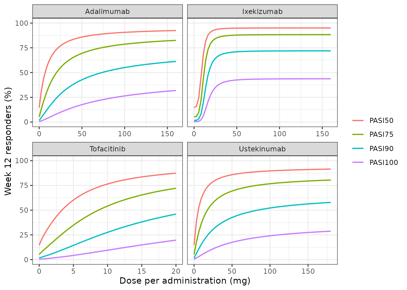
Replicates Figure 3 of Checchio 2017: model-predicted Week-12 PASI50/75/90/100 dose-response for four representative drugs. Dose 0 is the placebo arm of each study.
Figure 4: placebo-adjusted treatment effect
placeboRow <- rxode2::rxSolve(uiLand, makeArmData(arms |> filter(arm == "Placebo"), c(0, 12)),
                              returnType = "data.frame") |>
  filter(time == 12)

solLand |>
  transmute(arm,
            PASI75 = 100 * (prob_pasi75 - placeboRow$prob_pasi75),
            PASI90 = 100 * (prob_pasi90 - placeboRow$prob_pasi90)) |>
  pivot_longer(PASI75:PASI90, names_to = "endpoint", values_to = "effect") |>
  mutate(arm = stats::reorder(factor(arm), effect, FUN = max)) |>
  ggplot(aes(effect, arm, colour = endpoint)) +
  geom_point(size = 2) +
  labs(x = "Placebo-adjusted responders at Week 12 (percentage points)",
       y = NULL, colour = NULL) +
  theme_bw()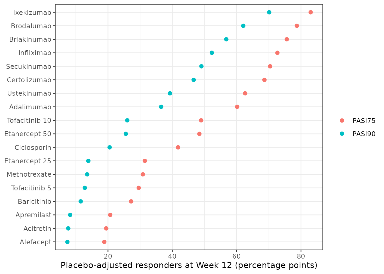
Replicates Figure 4 of Checchio 2017: Week-12 placebo-adjusted PASI75 and PASI90 treatment effect by drug at the clinical dose, typical 90 kg arm.
The source’s own headline comparison is that ixekizumab has the highest placebo-adjusted response, 88.2% - 5.5% = 82.7 percentage points for PASI75 and 70.0 for PASI90. The model gives 83.0 and 70.1.
ixe <- solLand |> filter(arm == "Ixekizumab")
stopifnot(
  abs(100 * (ixe$prob_pasi75 - placeboRow$prob_pasi75) - 82.7) < 1.5,
  abs(100 * (ixe$prob_pasi90 - placeboRow$prob_pasi90) - 70.0) < 1.5,
  # Ixekizumab must be the top agent on both endpoints, as the source reports.
  which.max(solLand$prob_pasi75) == which(solLand$arm == "Ixekizumab"),
  which.max(solLand$prob_pasi90) == which(solLand$arm == "Ixekizumab")
)
Figure 5: external validation of the PASI90 time course
The source’s most demanding check bridges the two models: the
longitudinal model, fitted to PASI75 only, is used to predict the
PASI90 time course by importing two scaling factors
from the landmark model – additively on the placebo term and
multiplicatively on the drug term. The packaged longitudinal model
carries those two imported constants as fixed() parameters
and emits prob_pasi90 as a secondary output.
solLong |>
  filter(time <= 24) |>
  select(arm, time, PASI75 = prob_pasi75, PASI90 = prob_pasi90) |>
  pivot_longer(PASI75:PASI90, names_to = "endpoint", values_to = "p") |>
  filter(arm %in% c("Ixekizumab", "Brodalumab", "Adalimumab", "Ustekinumab",
                    "Etanercept 50", "Methotrexate")) |>
  ggplot(aes(time, 100 * p, colour = arm, linetype = endpoint)) +
  geom_line(linewidth = 0.7) +
  labs(x = "Time (weeks)", y = "Responders (%)", colour = NULL, linetype = NULL) +
  coord_cartesian(ylim = c(0, 100)) +
  theme_bw()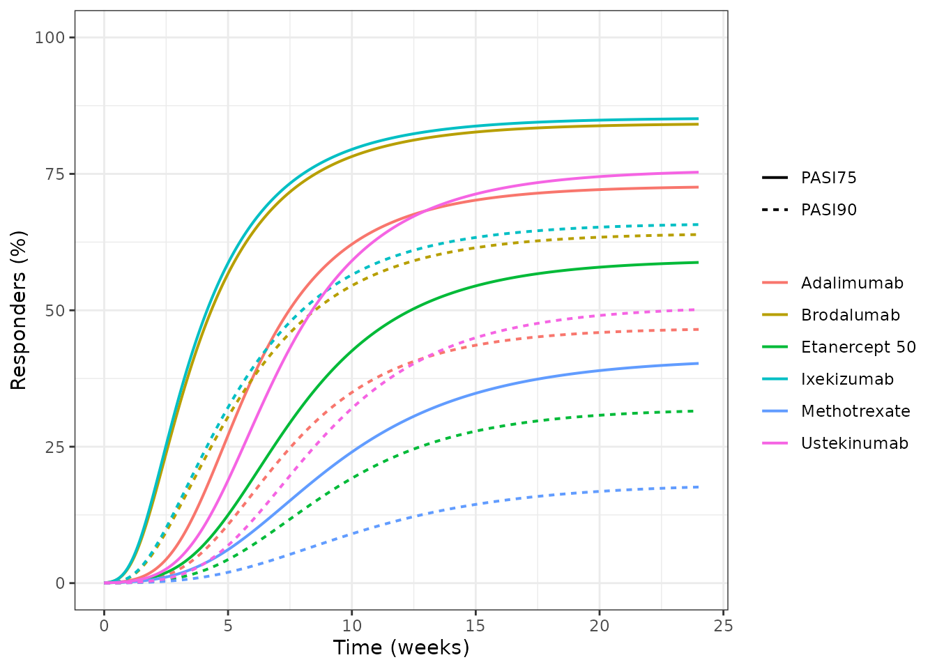
Replicates Figure 5 of Checchio 2017: PASI90 time course predicted by the longitudinal PASI75 model with the landmark PASI75-to-PASI90 scaling factors applied.
The bridge is checked against the landmark model rather than eyeballed: the two models were fitted independently, on different datasets, in different software, so their Week-12 PASI90 predictions agreeing is a real cross-validation. The source makes the same claim in prose (“There was close agreement between the estimates from the longitudinal model and the landmark model”), and the assertion below is what turns that claim into a test.
bridge <- solLong |>
  filter(time == 12) |>
  transmute(arm, longP90 = 100 * prob_pasi90) |>
  inner_join(cmpLand |> transmute(arm, landP90 = p90), by = "arm") |>
  mutate(diff = longP90 - landP90)

bridge |>
  transmute(Arm = arm, `Longitudinal PASI90 (%)` = round(longP90, 1),
            `Landmark PASI90 (%)` = round(landP90, 1),
            `Difference (pp)` = round(diff, 1)) |>
knitr::kable(caption = "Week-12 PASI90 from the two independently fitted models.")| Arm | Longitudinal PASI90 (%) | Landmark PASI90 (%) | Difference (pp) |
|---|---|---|---|
| Adalimumab | 39.8 | 38.1 | 1.6 |
| Certolizumab | 49.5 | 48.2 | 1.2 |
| Etanercept 25 | 13.2 | 15.5 | -2.3 |
| Etanercept 50 | 23.7 | 27.2 | -3.5 |
| Infliximab | 50.7 | 53.9 | -3.2 |
| Brodalumab | 58.4 | 63.7 | -5.3 |
| Ixekizumab | 60.3 | 71.7 | -11.4 |
| Secukinumab | 43.1 | 50.7 | -7.5 |
| Briakinumab | 55.8 | 58.4 | -2.6 |
| Ustekinumab | 38.9 | 40.9 | -2.0 |
| Methotrexate | 11.6 | 15.1 | -3.5 |
| Tofacitinib 5 | 18.6 | 14.4 | 4.2 |
| Tofacitinib 10 | 34.5 | 27.6 | 6.9 |
| Alefacept | 5.6 | 9.0 | -3.4 |
| Apremilast | 11.5 | 9.9 | 1.7 |
stopifnot(
  # PASI90 must sit below PASI75 at every time in every arm.
  all(solLong$prob_pasi90 <= solLong$prob_pasi75),
  # Nobody is a PASI90 responder at randomisation.
  all(solLong$prob_pasi90[solLong$time == 0] < 1e-3),
  # The two independently fitted models must agree on the central tendency.
  # Gated on the median and a robust quantile, not the extreme: the two models
  # used different study sets (57 vs 71 trials) and different software, so
  # per-drug scatter is expected and is not a transcription signal.
  abs(stats::median(bridge$diff)) < 5,
  stats::quantile(abs(bridge$diff), 0.9) < 15
)
cat(sprintf("Longitudinal vs landmark Week-12 PASI90: median difference %.1f pp, 90th percentile |difference| %.1f pp\n",
            stats::median(bridge$diff), stats::quantile(abs(bridge$diff), 0.9)))
#> Longitudinal vs landmark Week-12 PASI90: median difference -2.6 pp, 90th percentile |difference| 7.3 pp
Between-study variability
The longitudinal model is the one of the pair that carries usable random effects. Simulating study arms rather than patients shows the spread a trial designer should expect around the typical trajectory. The cohort is 150 arms, well inside the 200-per-arm cap.
rxode2::rxSetSeed(1234)
nArms <- 150
vpcArms <- arms |> filter(arm == "Ustekinumab") |> slice(rep(1, nArms))
vpcDat <- makeArmData(vpcArms, seq(0, 24, by = 1), nArm = 100)
vpcSol <- rxode2::rxSolve(uiLong, vpcDat, returnType = "data.frame")

vpcQ <- vpcSol |>
  group_by(time) |>
  summarise(lo = stats::quantile(prob_pasi75, 0.05),
            md = stats::median(prob_pasi75),
            hi = stats::quantile(prob_pasi75, 0.95), .groups = "drop")
typical <- solLong |> filter(arm == "Ustekinumab", time <= 24, time %% 1 == 0)

ggplot(vpcQ, aes(time)) +
  geom_ribbon(aes(ymin = 100 * lo, ymax = 100 * hi), fill = "grey80") +
  geom_line(aes(y = 100 * md), linewidth = 0.5, linetype = "dashed") +
  geom_line(data = typical, aes(time, 100 * prob_pasi75), linewidth = 1) +
  labs(x = "Time (weeks)", y = "PASI75 responders (%)") +
  coord_cartesian(ylim = c(0, 100)) +
  theme_bw()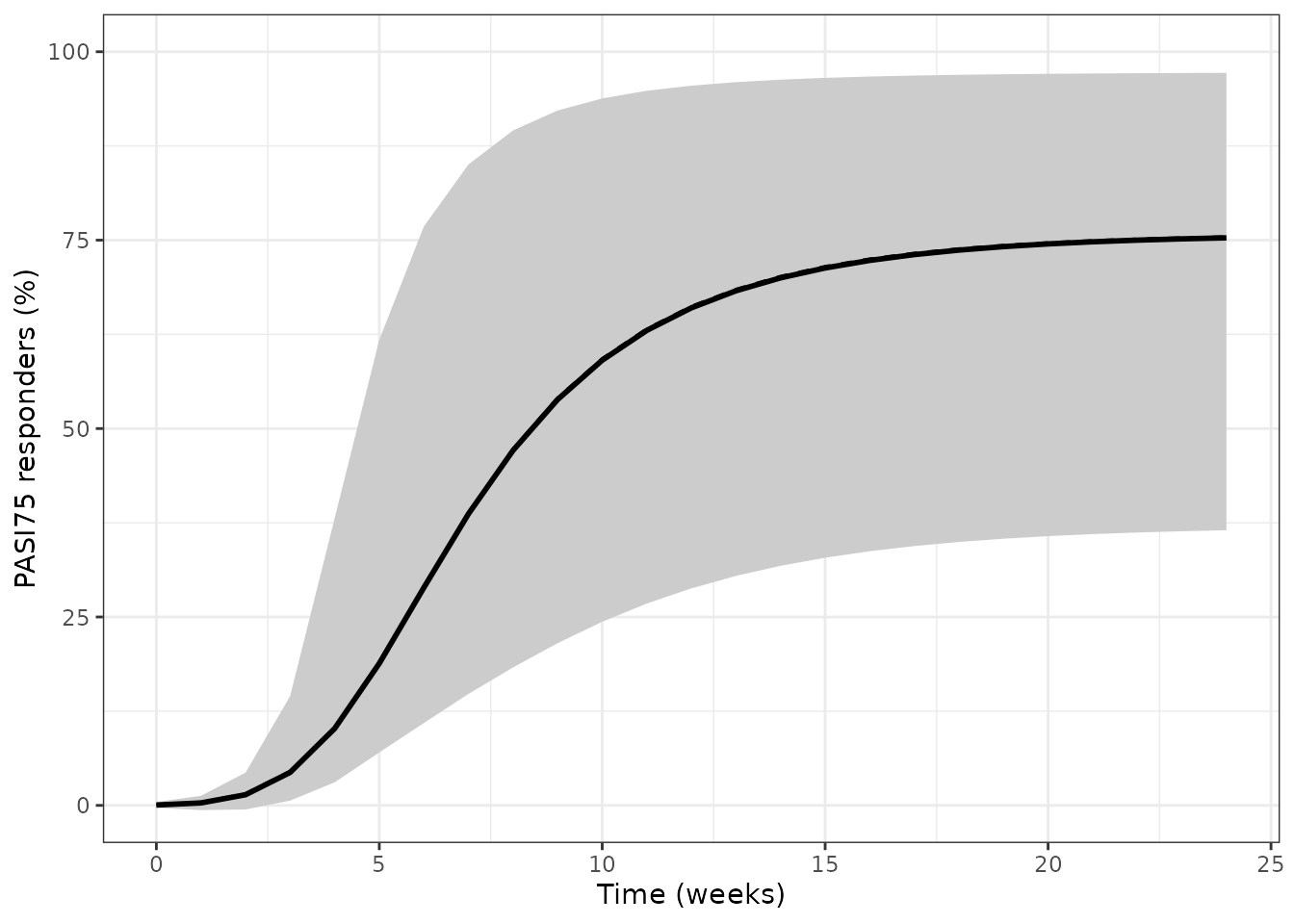
Simulated between-study spread of the ustekinumab 45 mg Q12W PASI75 time course (150 study arms of 100 patients each). The heavy line is the typical-value trajectory.
stopifnot(
  # The simulated arm distribution must bracket the typical trajectory: with
  # random effects centred at zero, the median arm should track it closely.
  # Gated on the central tendency, not on any simulated extreme, because the
  # draw is not reproducible across rxode2 versions.
  abs(100 * (vpcQ$md[vpcQ$time == 12] - typical$prob_pasi75[typical$time == 12])) < 5,
  # The spread must be non-degenerate and physically plausible.
  vpcQ$hi[vpcQ$time == 12] - vpcQ$lo[vpcQ$time == 12] > 0.05
)
Assumptions and deviations
Equation recovery
Every display equation is rasterised in the published PDF. Plain-text
extraction of the PDF loses all thirteen and yields no mathematics at
all. All thirteen equations were recovered with
pdftotext -layout. Wherever the recovered text was
ambiguous, the reading was settled by whether it reproduces the source’s
own published predictions, not by plausibility – the Table 1 and Table 2
comparisons above are that test.
The Hill coefficient is absent from the longitudinal model
Equation 4 carries an exponent and Methods says “The Hill coefficient was also tested in the model”, but no value appears anywhere in Supplementary Tables S1.1 or S1.2. It was therefore tested and not retained, and this model uses gamma = 1. That reading is confirmed numerically: every Week-4, Week-12 and ET50 value in Table 1 is reproduced. The landmark model does estimate a Hill coefficient, so the absence is a real difference between the two analyses rather than a reporting gap.
Dose is per administration
Neither paper table states the dose metric. It is settled arithmetically, by pairs of arms that share a single ED50 and differ only in dose: etanercept 25 and 50 mg twice weekly, and tofacitinib 5 and 10 mg twice daily. Only the per-administration reading reproduces both members of both pairs. Apremilast is the clearest single case: 30 mg reproduces its published values and 60 mg does not. Infliximab is mg/kg, per the Supplementary Table S1.1 footnote.
Certolizumab has no onset rate
Supplementary Table S1.1 reports no kdrug for
certolizumab, “Not estimated as only one study for certolizumab was
published”. The model uses the kdrug-to-infinity limit of Equation 4 –
zero before time zero, full effect after. That is not a choice among
plausible options: Table 1’s certolizumab Week-4 rate of 38.8% requires
a drug term of 4.102 logit units, which already exceeds that term’s own
ceiling of 4.097, so no finite onset rate can produce it. The limit
reproduces all four published certolizumab numbers.
Methotrexate, alefacept and the traditional oral agents are steps
Where the source could not estimate an ED50 it used a single-step
offset. In the longitudinal model that applies to methotrexate and
alefacept; in the landmark model to methotrexate, ciclosporin and
acitretin. For those agents the model is only valid at the clinical dose
in the arm table, and > 0 is the only thing read from
the dose column. Predicting a different dose of those agents from these
models is not supported.
The alefacept route
Supplementary Table 2 carries an IV offset on the alefacept ED50 with
a non-IV (intramuscular) reference. The source’s own Table 2 prediction
for “Alefacept 10 mg QW” is reproduced by the IV branch
(24.1% against a published 22.7%), not the IM branch (11.8%).
ROUTE_IV = 1 is therefore required to reproduce any
published alefacept number, and the arm table above sets it. The source
does not state which route its typical-patient simulation assumed; the
arithmetic does.
Two values are back-solved, not printed
e0_trial and led50_briakinumab are not in
the paper or its supplement and are recovered by inverting the source’s
own Table 2 predictions through its own Equations 5-8, as shown above
and re-derived at render time. Neither is a value imported from outside
the paper. The evidence that the inversion is sound is that
e0_trial is over-determined 36-to-1 with small unstructured
residuals, and that it independently reproduces the typical placebo
rates implied by Table 2’s separate “difference from placebo”
columns.
Random-effect and residual scale in the longitudinal model
Supplementary Table S1.2 labels its variance rows “omega”, “sigma”
and “sigma corr” while the Methods text names the variances “omega
squared” and “sigma squared”, so the printed numbers could be read as
variances or as standard deviations. They are read here as
variances, for two reasons. The table is headed “Common
Parameter Estimates from NONMEM Output”, and a NONMEM
$OMEGA estimate is a variance. And the SD reading is
physically too tight: it would confine the Week-12 placebo PASI75 to
4.0-5.5% across a one-SD band, whereas published psoriasis placebo arms
span roughly 1-8% and the source’s own landmark analysis measures an
I-squared of 82% for between-study placebo heterogeneity. The variance
reading gives 2.3-9.4%.
This choice changes no typical-value prediction – every comparison in this vignette is unaffected – only the simulated between-study spread in the section above. For the two residual terms it is nearly immaterial even there: the total multiplier on the binomial standard error is 1.28 under the variance reading and 1.21 under the SD reading, and only the split between the two terms differs.
The landmark model has no variability
Equation 5 carries an endpoint-specific random effect and the Methods
describe within-study and between-arm correlation terms, but
Supplementary Table 2 tabulates only fixed effects: no variance, no
correlation matrix, and no residual. None is encoded, because inventing
one would be unauditable. The landmark model therefore produces
typical-value arm predictions only, and its ini() carries a
fixed placeholder residual purely so the likelihood machinery accepts it
for forward simulation. Use the longitudinal model when between-study
spread is needed.
The practical consequence is visible in the Table 2 comparison: the source’s published numbers are means over 1,000 simulations including that random effect, so the two arms with the largest residuals differ from the typical-value prediction in the direction Jensen’s inequality requires.
ET90 runs short for the slower drugs
Reproduced ET50 matches every published value to within 0.3 weeks. ET90 runs about one week short for the slowest drugs, most likely because the source evaluated the maximal treatment effect at a finite horizon rather than at infinity. ET50 is the metric the source’s Discussion uses; the ET90 deviation is recorded here rather than tuned away.
Residual weighting is applied inside the model
Most of this package’s MBMA extractions store the residual SD
unweighted and leave the 1/sqrt(N) arm weighting to
downstream code. This one carries N_ARM as a covariate
column and applies the binomial standard error
W = sqrt(Pr*(1-Pr)/N_ARM) inside model(),
because the arm-level correlated term of Equation 13 is a random
effect whose SD varies from arm to arm, and a per-arm random-effect
SD cannot be reproduced by rescaling the output of a single
rxSolve().
Scope
Both models predict study-arm mean responder rates, not individual-patient outcomes. The source is explicit that the body weight effect is an aggregate-level association whose magnitude is probably attenuated, and that its attribution to the placebo component “should not be interpreted in a mechanistic context”. Neither model has a PK layer, so neither can be driven by exposure.
Bootstrap versus final estimates
The Results text quotes the body weight effects as -0.193 and -0.867, which are medians of a 1,000-replicate nonparametric bootstrap. Supplementary Table S1.2 gives the NONMEM final estimates, -0.198 and -0.834, and those are what the model uses. Both pairs exclude zero and agree in sign and magnitude.