Idiopathic pulmonary fibrosis percent-predicted FVC MBMA (Chan 2017)
Source:vignettes/articles/Chan_2017_ipf_fvc.Rmd
Chan_2017_ipf_fvc.RmdModel and source
- Citation: Chan P, Bax L, Chen C, Zhang N, Huang SP, Soares H, Rosen G, AbuTarif M. Model-based Meta-Analysis on the Efficacy of Pharmacological Treatments for Idiopathic Pulmonary Fibrosis. CPT Pharmacometrics Syst Pharmacol. 2017;6(10):695-704. doi:10.1002/psp4.12227. Final parameter estimates are in Table 2; the treatment-effect ranking is duplicated in Figure 2; the model equation is Eq. 1 with the time-course and baseline-covariate forms given in the Table 2 note.
- Description: MBMA. Longitudinal model-based meta-analysis of the placebo-corrected change from baseline in percent-predicted forced vital capacity (%predicted FVC) for 15 treatment regimens in idiopathic pulmonary fibrosis, fit by maximum likelihood (R 3.1.2, nlme::gnls) to arm-level summary data from 43 arms (148 arm-timepoints, 4,919 subjects) in 20 published trials with treatment durations of 8-104 weeks (Chan 2017). Each treatment carries its own maximum effect Emax in %predicted FVC; a single shared empirical time course 1 - exp(-kel * time) governs how fast that maximum is approached (kel = exp(lambda) = 0.0417 /week, so 50% of the maximum at 16.6 weeks and 90% at 55 weeks); and the arm’s mean baseline %predicted FVC scales the whole treatment effect through the power term (FVC_PCTPRED / 74)^1.48. Pirfenidone is the only treatment with a dose-response: a step function selected by DOSE_HIGH gives 2.42 at 1,197 mg/day and 3.87 at 2,403 mg/day. Pirfenidone and nintedanib were the only regimens whose 95% CI excluded zero. CRITICAL SCOPE LIMIT: the output fvcppcfb is the PLACEBO-CORRECTED change from baseline, i.e. the active-minus-placebo difference only. Chan 2017 modelled the placebo arm NONPARAMETRICALLY – one free estimate per trial per timepoint, deliberately so that no distributional assumption was imposed on the highly variable IPF placebo response – and those per-trial placebo estimates are not tabulated in the paper. This model therefore CANNOT produce an absolute %predicted FVC trajectory; to reproduce a figure like Chan 2017 Figure 3 the user must supply the trial’s own observed placebo arm. Suitable simulation scope is the study-arm-mean placebo-corrected treatment effect, NOT individual-patient FVC.
- Article: https://doi.org/10.1002/psp4.12227
- Open-access full text: https://www.ncbi.nlm.nih.gov/pmc/articles/PMC5658284/
Chan 2017 is a longitudinal model-based meta-analysis (MBMA) of the change from baseline in percent-predicted forced vital capacity (%predicted FVC) in idiopathic pulmonary fibrosis (IPF). It pools arm-level summary data from 20 published trials to compare 15 treatment regimens indirectly, at a time when pirfenidone and nintedanib had just become the first two FDA-approved IPF therapies and no head-to-head trial existed.
What this model produces, and what it does not
This is the single most important thing to understand before using the model.
Chan 2017 Eq. 1 is
dY_ijt = E0_it + f(theta_ki) + eta_ij + eps_ijtwhere E0_it is the placebo response for trial
i at time t. Chan 2017 estimated that term
nonparametrically – one free parameter per trial per
timepoint – deliberately, so that no distributional assumption was
imposed on the IPF placebo response, which is highly variable across
trials. Those per-trial placebo estimates are not tabulated in
the paper.
What the paper does tabulate is everything in
f(theta_ki): the 15 treatment Emax values, the shared time
course, and the baseline-lung-function covariate. So the packaged model
reproduces
fvcppcfb = Emax_treatment * (1 - exp(-kel * time)) * (FVC_PCTPRED / 74)^embasewhich is exactly the placebo-corrected change from baseline – the active-minus-placebo difference plotted in Chan 2017 Figures 2, 4 and 5, and the vertical gap between the fitted curves of Figure 3.
| You can simulate | You cannot simulate |
|---|---|
| The placebo-corrected treatment effect of any of the 15 regimens, over time, at any arm baseline | The absolute %predicted FVC trajectory |
| The arm-level contrast that Figures 2, 4 and 5 report | The placebo arm’s own decline |
| Study-arm-mean responses | Individual-patient FVC |
To draw a figure like Chan 2017 Figure 3, a user must supply the trial’s own observed placebo arm and add this model’s output to it.
Population
The analysis dataset comprises 43 arms and 148 arm-timepoints from 4,919 subjects in 20 trials (Chan 2017 Table 1), selected from a larger 40-citation / 32-trial database built by a PRISMA-style systematic review of PubMed plus the FDA and ClinicalTrials.gov websites (search run September 2015). Seventeen of the 20 trials were double-blinded and placebo-controlled, and none had stratified data within arms. Treatment durations ranged from 8 to 104 weeks. Trials were conducted in Europe, North America and Australia; Chan 2017 notes that none was conducted in Asia.
Placebo contributed the largest single block (17 arms, 63 timepoints, 2,035 subjects). The most-studied active treatments were interferon gamma (4 arms, 607 subjects), nintedanib (3 arms, 723 subjects) and pirfenidone (4 arms, 710 subjects). Eight treatments contributed longitudinal data; the remaining six contributed a single timepoint each.
Baseline %predicted FVC – the only covariate retained – had an approximate median of 74% across the dataset, which is the model’s normalising constant. Weight, height and body mass index were not available: more than 60% of trial arms had missing values, so Chan 2017 did not impute them.
The same information is available programmatically:
pop <- rxode2::rxode(readModelDb("Chan_2017_ipf_fvc_mbma"))$population
#> ℹ parameter labels from comments will be replaced by 'label()'
str(pop[c("n_subjects", "n_studies", "n_arms", "n_observations", "regions")])
#> List of 5
#>  $ n_subjects    : int 4919
#>  $ n_studies     : int 20
#>  $ n_arms        : int 43
#>  $ n_observations: int 148
#>  $ regions       : chr "Europe, North America and Australia; Chan 2017 Results notes that none of the 20 trials was conducted in Asia"
Source trace
Every ini() entry in
inst/modeldb/therapeuticArea/Chan_2017_ipf_fvc_mbma.R
carries an in-file comment naming its source location. They are
collected here for review.
| Equation / parameter | Value | Source location |
|---|---|---|
Model equation dY = E0 + f(theta) + eta + eps
|
n/a | Eq. 1 (Methods, “Model development”) |
Time course 1 - exp(-lambda*time)
|
n/a | Table 2 note; Results, “Model development” |
Baseline covariate (baseline %predFVC / 74)^embase
|
n/a | Table 2 note |
emax_ifngamma |
-0.618 | Table 2 “Interferon-gamma treatment”; Figure 2 |
emax_colchicine |
-7.63 | Table 2 “Colchicine treatment”; Figure 2 |
emax_prednisone |
-11.9 | Table 2 “Prednisone treatment”; Figure 2 |
emax_sildenafil |
2.67 | Table 2 “Sildenafil treatment”; Figure 2 |
emax_bosentan |
1.75 | Table 2 “Bosentan treatment”; Figure 2 |
emax_ambrisentan |
-2.03 | Table 2 “Ambrisentan treatment”; Figure 2 |
emax_acetylcysteine |
-0.0568 | Table 2 “N-acetylcysteine treatment”; Figure 2 |
emax_warfarin |
-0.276 | Table 2 “Warfarin treatment”; Figure 2 |
emax_etanercept |
1.47 | Table 2 “Etanercept treatment”; Figure 2 |
emax_azathioprine |
5.89 | Table 2 “Azathioprine treatment”; Figure 2 |
emax_cotrimoxazole |
0.172 | Table 2 “Co-trimoxazole treatment”; Figure 2 |
emax_nintedanib |
3.31 | Table 2 “Nintedanib treatment”; Figure 2 |
emax_pirfenidone_low |
2.42 | Table 2 “Pirfenidone 1,197 mg/day treatment”; Figure 2 |
emax_pirfenidone_high |
3.87 | Table 2 “Pirfenidone 2,403 mg/day treatment”; Figure 2 |
emax_prm151 |
12.5 | Table 2 “PRM-151 treatment”; Figure 2 |
lkel (lambda) |
-3.18 | Table 2 “Time-varying effect (lambda)”; t50/t90 in Results |
e_fvc_pctpred_emax (embase) |
1.48 | Table 2 “Baseline FVC effect (embase)” – see Errata |
eta_arm_fvcppcfb |
1.07e-6 | Table 2 “Between trial-arm variability” |
addSd |
fixed(1) | Eq. 1 – unit-weight scale; no sigma is tabulated |
All 15 Emax values appear twice in the paper – in Table 2 and in the Figure 2 ranking plot – and the two agree to every printed digit. That duplication is the cross-check used for this block.
Setting up the model
mod_full <- readModelDb("Chan_2017_ipf_fvc_mbma")()

# Every figure below is a TYPICAL-VALUE prediction, so the between-arm random
# effect and the unit-weight residual are both zeroed. This is not cosmetic:
# the packaged addSd is the residual at UNIT STUDY WEIGHT, and applying it
# unscaled would add a 1.0 %predicted-FVC error to every point, which is the
# wrong magnitude for every real arm in the dataset (see Assumptions).
mod_typ <- rxode2::zeroRe(mod_full)

# The 15 regimens, as indicator settings. Exactly one indicator is 1 per arm;
# DOSE_HIGH is only meaningful when PIRFENIDONE is 1.
regimens <- tibble::tribble(
  ~treatment,                 ~indicator,          ~DOSE_HIGH, ~emax,
  "PRM-151",                  "PRM151",                    0L,  12.5,
  "Azathioprine",             "AZATHIOPRINE",              0L,   5.89,
  "Pirfenidone 2403 mg/day",  "PIRFENIDONE",               1L,   3.87,
  "Nintedanib 300 mg/day",    "NINTEDANIB",                0L,   3.31,
  "Sildenafil",               "SILDENAFIL",                0L,   2.67,
  "Pirfenidone 1197 mg/day",  "PIRFENIDONE",               0L,   2.42,
  "Bosentan",                 "BOSENTAN",                  0L,   1.75,
  "Etanercept",               "ETANERCEPT",                0L,   1.47,
  "Co-trimoxazole",           "COTRIMOXAZOLE",             0L,   0.172,
  "N-acetylcysteine",         "ACETYLCYSTEINE",            0L,  -0.0568,
  "Warfarin",                 "WARFARIN",                  0L,  -0.276,
  "Interferon gamma",         "INTERFERON_GAMMA",          0L,  -0.618,
  "Ambrisentan",              "AMBRISENTAN",               0L,  -2.03,
  "Colchicine",               "COLCHICINE",                0L,  -7.63,
  "Prednisone",               "PREDNISONE",                0L, -11.9
)

all_indicators <- c(
  "NINTEDANIB", "PIRFENIDONE", "PRM151", "INTERFERON_GAMMA", "COLCHICINE",
  "PREDNISONE", "SILDENAFIL", "BOSENTAN", "AMBRISENTAN", "ACETYLCYSTEINE",
  "WARFARIN", "ETANERCEPT", "AZATHIOPRINE", "COTRIMOXAZOLE"
)

# Build one arm: a time grid, all 14 indicators zeroed except the active one,
# the pirfenidone dose step, and the arm's baseline %predicted FVC.
build_arm <- function(tgrid, indicator, dose_high, fvc_pctpred, label,
                      id_offset = 0L) {
  ev <- as.data.frame(rxode2::et(tgrid))
  ev$id <- id_offset + 1L
  for (nm in all_indicators) ev[[nm]] <- 0L
  if (!is.na(indicator)) ev[[indicator]] <- 1L
  ev$DOSE_HIGH <- as.integer(dose_high)
  ev$FVC_PCTPRED <- fvc_pctpred
  ev$treatment <- label
  ev
}
Internal-consistency gates
Before replicating any figure, two checks confirm the model was transcribed on the scale the paper intended. Both compare against numbers Chan 2017 prints in its own Results text, and both are deterministic, so they are asserted tightly.
Gate 1 – lambda is on the log scale
Chan 2017 Table 2 reports the time-varying effect as
lambda = -3.18 and the note writes the time course as
1-exp(-lambda*time), which reads as if lambda were the rate
constant. It cannot be: a rate of -3.18 /week makes
1 - exp(+3.18*t) diverge to -Inf. The Results
text supplies the disambiguation – 50% of maximum at 16.5 weeks, 90% “at
56 weeks” – and only kel = exp(lambda) reproduces both.
kel <- exp(-3.18)
t50 <- log(2) / kel
t90 <- log(10) / kel

gate1 <- tibble::tibble(
  Quantity = c("kel (1/week)", "Time to 50% of maximum (weeks)",
               "Time to 90% of maximum (weeks)"),
  Model = c(kel, t50, t90),
  Published = c(NA, 16.5, 56),
  Source = c("exp(lambda), lambda = -3.18 (Table 2)",
             "Results: 'time to 50% maximum efficacy of 16.5 weeks'",
             "Results: '90% of maximum response ... at 56 weeks'")
)
knitr::kable(gate1, digits = 4,
caption = "Gate 1: the log-scale reading of lambda reproduces the paper's own onset timings.")| Quantity | Model | Published | Source |
|---|---|---|---|
| kel (1/week) | 0.0416 | NA | exp(lambda), lambda = -3.18 (Table 2) |
| Time to 50% of maximum (weeks) | 16.6679 | 16.5 | Results: ‘time to 50% maximum efficacy of 16.5 weeks’ |
| Time to 90% of maximum (weeks) | 55.3697 | 56.0 | Results: ‘90% of maximum response … at 56 weeks’ |
# Deterministic closed form vs two printed values; the paper rounds to 3 and 2
# significant figures respectively, so the tolerances below are rounding-width,
# not fitted. The alternative (linear) reading of lambda gives t50 = 0.22 weeks
# and would miss by a factor of 75, so this gate discriminates decisively.
stopifnot(
  abs(t50 - 16.5) < 0.5,
  abs(t90 - 56) < 1.5
)
Gate 2 – each indicator selects its own Emax
At the reference baseline of 74% predicted FVC and at large time, the model must return each treatment’s tabulated Emax exactly. This catches a mis-wired indicator, a transposed value, or a covariate term that does not collapse to 1 at the reference.
ev_plateau <- dplyr::bind_rows(lapply(seq_len(nrow(regimens)), function(i) {
  build_arm(
    tgrid = 2000, indicator = regimens$indicator[i],
    dose_high = regimens$DOSE_HIGH[i], fvc_pctpred = 74,
    label = regimens$treatment[i], id_offset = i
  )
}))
stopifnot(!anyDuplicated(unique(ev_plateau[, c("id", "time")])))

sim_plateau <- rxode2::rxSolve(mod_typ, events = ev_plateau,
                               keep = c("treatment")) |>
  as.data.frame()
#> ℹ omega/sigma items treated as zero: 'eta_arm_fvcppcfb'
#> Warning: multi-subject simulation without without 'omega'

gate2 <- sim_plateau |>
  dplyr::select(treatment, Model = fvcppcfb) |>
  dplyr::left_join(regimens |> dplyr::select(treatment, Published = emax),
                   by = "treatment") |>
  dplyr::mutate(Difference = Model - Published) |>
  dplyr::arrange(dplyr::desc(Published))

knitr::kable(gate2, digits = 6,
caption = "Gate 2: plateau effect at the 74% reference baseline vs Chan 2017 Table 2.")| treatment | Model | Published | Difference |
|---|---|---|---|
| PRM-151 | 12.5000 | 12.5000 | 0 |
| Azathioprine | 5.8900 | 5.8900 | 0 |
| Pirfenidone 2403 mg/day | 3.8700 | 3.8700 | 0 |
| Nintedanib 300 mg/day | 3.3100 | 3.3100 | 0 |
| Sildenafil | 2.6700 | 2.6700 | 0 |
| Pirfenidone 1197 mg/day | 2.4200 | 2.4200 | 0 |
| Bosentan | 1.7500 | 1.7500 | 0 |
| Etanercept | 1.4700 | 1.4700 | 0 |
| Co-trimoxazole | 0.1720 | 0.1720 | 0 |
| N-acetylcysteine | -0.0568 | -0.0568 | 0 |
| Warfarin | -0.2760 | -0.2760 | 0 |
| Interferon gamma | -0.6180 | -0.6180 | 0 |
| Ambrisentan | -2.0300 | -2.0300 | 0 |
| Colchicine | -7.6300 | -7.6300 | 0 |
| Prednisone | -11.9000 | -11.9000 | 0 |
Replicate Figure 2 – treatment ranking
Chan 2017 Figure 2 ranks the 15 regimens by their maximum effect. Because Gate 2 has already shown the plateau reproduces Table 2 exactly, this figure is a presentation of the same numbers with their published confidence intervals.
fig2 <- tibble::tribble(
  ~treatment,                ~est,     ~lo,    ~hi,
  "PRM-151",                  12.5,   -5.13,  30.1,
  "Azathioprine",              5.89,  -4.14,  15.9,
  "Pirfenidone 2403 mg/day",   3.87,   2.68,   5.06,
  "Nintedanib 300 mg/day",     3.31,   2.15,   4.47,
  "Sildenafil",                2.67,  -7.15,  12.5,
  "Pirfenidone 1197 mg/day",   2.42,   0.733,  4.11,
  "Bosentan",                  1.75,  -4.37,   7.86,
  "Etanercept",                1.47,  -2.3,    5.24,
  "Co-trimoxazole",            0.172, -3.72,   4.07,
  "N-acetylcysteine",         -0.0568,-2.01,   1.9,
  "Warfarin",                 -0.276, -4.89,   4.33,
  "Interferon gamma",         -0.618, -2.46,   1.23,
  "Ambrisentan",              -2.03,  -4.18,   0.126,
  "Colchicine",               -7.63, -13,     -2.3,
  "Prednisone",              -11.9,  -25.8,    1.95
) |>
  dplyr::mutate(
    significant = lo > 0 | hi < 0,
    treatment = factor(treatment, levels = rev(treatment))
  )

ggplot(fig2, aes(x = est, y = treatment, colour = significant)) +
  geom_vline(xintercept = 0, linetype = "dashed", colour = "grey50") +
  geom_pointrange(aes(xmin = lo, xmax = hi)) +
  scale_colour_manual(values = c(`TRUE` = "firebrick", `FALSE` = "grey35"),
                      labels = c(`TRUE` = "CI excludes 0", `FALSE` = "CI includes 0"),
                      name = NULL) +
  labs(x = "Maximum effect (%predicted FVC)", y = NULL,
       title = "Figure 2 - maximum treatment effect by regimen",
       caption = "Replicates Figure 2 of Chan 2017.")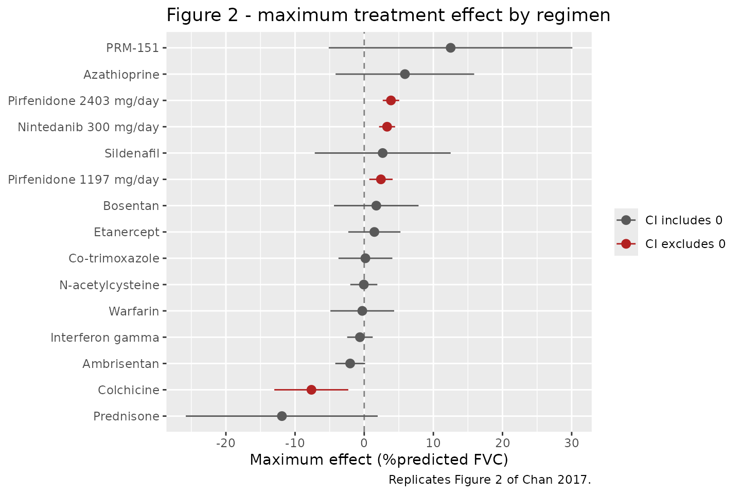
Replicates Figure 2 of Chan 2017: model-estimated maximum (saturable) effect and 95% CI for each active treatment. Only pirfenidone and nintedanib have CIs excluding zero.
# The paper's headline claim: exactly two regimens have CIs excluding the null,
# and both are positive. Chan 2017 Results: "pirfenidone and nintedanib were
# the only drugs identified to have statistically significant positive
# treatment effects".
sig <- fig2$treatment[fig2$significant]
stopifnot(
  setdiff(as.character(sig),
          c("Pirfenidone 2403 mg/day", "Nintedanib 300 mg/day",
            "Pirfenidone 1197 mg/day", "Colchicine")) |> length() == 0,
  all(c("Pirfenidone 2403 mg/day", "Nintedanib 300 mg/day") %in% as.character(sig))
)
Note that colchicine’s CI also excludes zero, but on the negative side; the paper’s claim is about significant positive effects, which pirfenidone (both doses) and nintedanib alone satisfy.
Replicate Figure 5 – baseline %predicted FVC on the time course
Chan 2017 Figure 5 simulates nintedanib and pirfenidone over 52 weeks
at two baseline lung-function levels, the observed medians of the
stratified low and high baseline groups. The figure legend labels them
FVC=67 and FVC=76.
This figure is also the decisive evidence for which
embase value belongs to the final model – see the Errata
below.
tgrid5 <- seq(0, 52, by = 0.5)

fig5_design <- tidyr::expand_grid(
  tibble::tibble(
    treatment = c("Nintedanib", "Pirfenidone"),
    indicator = c("NINTEDANIB", "PIRFENIDONE"),
    DOSE_HIGH = c(0L, 1L)
  ),
  FVC_PCTPRED = c(67, 76)
)

ev_fig5 <- dplyr::bind_rows(lapply(seq_len(nrow(fig5_design)), function(i) {
  ev <- build_arm(
    tgrid = tgrid5, indicator = fig5_design$indicator[i],
    dose_high = fig5_design$DOSE_HIGH[i],
    fvc_pctpred = fig5_design$FVC_PCTPRED[i],
    label = fig5_design$treatment[i], id_offset = i
  )
  ev$baseline <- paste0("FVC=", fig5_design$FVC_PCTPRED[i])
  ev
}))
stopifnot(!anyDuplicated(unique(ev_fig5[, c("id", "time")])))

sim_fig5 <- rxode2::rxSolve(mod_typ, events = ev_fig5,
                            keep = c("treatment", "baseline")) |>
  as.data.frame()
#> ℹ omega/sigma items treated as zero: 'eta_arm_fvcppcfb'
#> Warning: multi-subject simulation without without 'omega'

ggplot(sim_fig5, aes(time, fvcppcfb, colour = baseline)) +
  geom_line(linewidth = 0.9) +
  facet_wrap(~treatment) +
  scale_colour_manual(values = c("FVC=67" = "black", "FVC=76" = "firebrick")) +
  coord_cartesian(ylim = c(-1, 5)) +
  labs(x = "Time (week)",
       y = "Placebo-corrected change from baseline\nof percent predicted FVC (percent)",
       colour = NULL,
       title = "Figure 5 - effect of baseline %predicted FVC",
       caption = "Replicates Figure 5 of Chan 2017 (median line only; the paper also shows a 95% prediction interval).")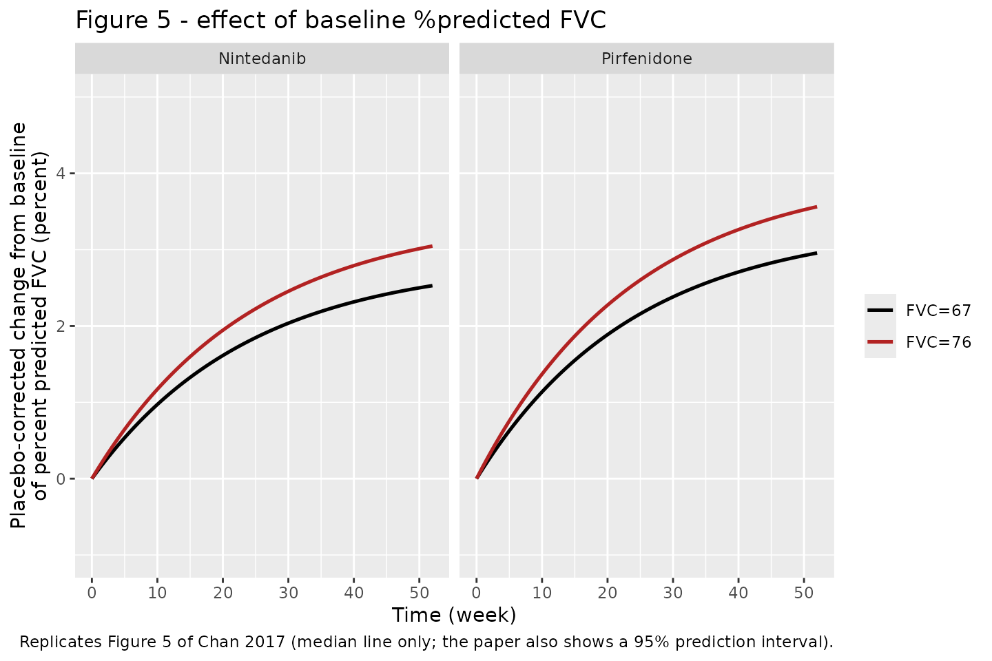
Replicates Figure 5 of Chan 2017: predicted placebo-corrected change from baseline %predicted FVC for nintedanib 300 mg/day and pirfenidone 2403 mg/day, at baseline %predicted FVC of 67 and 76.
Quantitative comparison against Figure 5
The published figure has no numeric annotations, so the reference column below was read off the rendered panels at 250 dpi. Reading precision is roughly +/- 0.1 %predicted FVC, which is what the tolerances allow for.
end5 <- sim_fig5 |>
  dplyr::filter(time == 52) |>
  dplyr::select(treatment, baseline, Model = fvcppcfb)

digitised <- tibble::tribble(
  ~treatment,    ~baseline,  ~Digitised,
  "Nintedanib",  "FVC=67",   2.40,
  "Nintedanib",  "FVC=76",   3.00,
  "Pirfenidone", "FVC=67",   2.85,
  "Pirfenidone", "FVC=76",   3.50
)

cmp5 <- end5 |>
  dplyr::left_join(digitised, by = c("treatment", "baseline")) |>
  dplyr::mutate(Difference = Model - Digitised)

cmp5 |>
  dplyr::rename("Treatment" = treatment, "Baseline" = baseline,
                "Model (week 52)" = Model,
                "Digitised from Fig 5" = Digitised) |>
  knitr::kable(digits = 3,
caption = "Model vs values digitised from Chan 2017 Figure 5 at week 52.")| Treatment | Baseline | Model (week 52) | Digitised from Fig 5 | Difference |
|---|---|---|---|---|
| Nintedanib | FVC=67 | 2.529 | 2.40 | 0.129 |
| Nintedanib | FVC=76 | 3.047 | 3.00 | 0.047 |
| Pirfenidone | FVC=67 | 2.956 | 2.85 | 0.106 |
| Pirfenidone | FVC=76 | 3.563 | 3.50 | 0.063 |
# Level agreement, at the resolution the panels can be read to.
stopifnot(max(abs(cmp5$Difference)) < 0.35)
The ratio between the two baseline curves is the sharper test, because everything except the covariate term cancels:
effect(FVC = 76) / effect(FVC = 67) = (76 / 67)^embasewhich is 1.21 for embase = 1.48 and 1.63 for the
alternative value of 3.86 printed in the Results text.
ratio <- cmp5 |>
  dplyr::select(treatment, baseline, Model) |>
  tidyr::pivot_wider(names_from = baseline, values_from = Model) |>
  dplyr::mutate(Ratio = `FVC=76` / `FVC=67`)

ratio_digitised <- 3.00 / 2.40   # nintedanib, read from Figure 5
ratio_if_148 <- (76 / 67)^1.48
ratio_if_386 <- (76 / 67)^3.86

tibble::tibble(
  Source = c("Model as packaged (embase = 1.48)",
             "Closed form with embase = 1.48",
             "Closed form with embase = 3.86 (Results text)",
             "Digitised from Figure 5 (nintedanib)"),
  `FVC=76 / FVC=67` = c(ratio$Ratio[ratio$treatment == "Nintedanib"],
                        ratio_if_148, ratio_if_386, ratio_digitised)
) |>
  knitr::kable(digits = 3,
caption = "The baseline-curve ratio discriminates the two candidate embase values.")| Source | FVC=76 / FVC=67 |
|---|---|
| Model as packaged (embase = 1.48) | 1.205 |
| Closed form with embase = 1.48 | 1.205 |
| Closed form with embase = 3.86 (Results text) | 1.627 |
| Digitised from Figure 5 (nintedanib) | 1.250 |
# The packaged model must match its own closed form exactly, and must sit far
# from the 3.86 alternative. The midpoint of the two candidate ratios is 1.42;
# the bound below is on the 1.48 side of it and rejects 3.86 by a wide margin.
stopifnot(
  abs(ratio$Ratio - ratio_if_148) < 1e-8,
  all(ratio$Ratio < 1.40),
  ratio_if_386 > 1.40
)
Replicate Figure 3 – the fitted active-minus-placebo gap
Chan 2017 Figure 3 plots two representative trials with their fitted
curves. The panels annotate each trial’s own baseline:
base=76.2 for CAPACITY-2 (PIPF-004) and
base=74.2 for TOMORROW. The model cannot draw the curves
themselves (they include the nonparametric placebo), but the
vertical gap between an active curve and the placebo
curve in each panel is exactly what this model predicts.
fig3_design <- tibble::tribble(
  ~trial,              ~treatment,                ~indicator,    ~DOSE_HIGH, ~base, ~week, ~digitised_gap,
  "CAPACITY-2",        "Pirfenidone 2403 mg/day", "PIRFENIDONE",         1L,  76.2,    24,  2.55,
  "CAPACITY-2",        "Pirfenidone 1197 mg/day", "PIRFENIDONE",         0L,  76.2,    24,  1.41,
  "TOMORROW",          "Nintedanib 300 mg/day",   "NINTEDANIB",          0L,  74.2,    52,  NA
)

ev_fig3 <- dplyr::bind_rows(lapply(seq_len(nrow(fig3_design)), function(i) {
  build_arm(
    tgrid = fig3_design$week[i], indicator = fig3_design$indicator[i],
    dose_high = fig3_design$DOSE_HIGH[i], fvc_pctpred = fig3_design$base[i],
    label = paste(fig3_design$trial[i], fig3_design$treatment[i]),
    id_offset = i
  )
}))

sim_fig3 <- rxode2::rxSolve(mod_typ, events = ev_fig3,
                            keep = c("treatment")) |>
  as.data.frame()
#> ℹ omega/sigma items treated as zero: 'eta_arm_fvcppcfb'
#> Warning: multi-subject simulation without without 'omega'

cmp3 <- fig3_design |>
  dplyr::mutate(Model = sim_fig3$fvcppcfb) |>
  dplyr::select(Trial = trial, Treatment = treatment,
                `Baseline %predFVC` = base, Week = week,
                `Model gap` = Model, `Digitised gap` = digitised_gap)

knitr::kable(cmp3, digits = 3,
caption = "Active-minus-placebo gap in Chan 2017 Figure 3, model vs values digitised from the published panels.")| Trial | Treatment | Baseline %predFVC | Week | Model gap | Digitised gap |
|---|---|---|---|---|---|
| CAPACITY-2 | Pirfenidone 2403 mg/day | 76.2 | 24 | 2.552 | 2.55 |
| CAPACITY-2 | Pirfenidone 1197 mg/day | 76.2 | 24 | 1.596 | 1.41 |
| TOMORROW | Nintedanib 300 mg/day | 74.2 | 52 | 2.941 | NA |
# Only the two CAPACITY-2 arms were read off the panel; TOMORROW's last visit
# is partly obscured in the crop and is shown for completeness without a gate.
gated3 <- cmp3[!is.na(cmp3$`Digitised gap`), ]
stopifnot(max(abs(gated3$`Model gap` - gated3$`Digitised gap`)) < 0.35)
The 2,403 mg/day arm agrees to three significant figures
(3.87 * 0.632 * 1.044 = 2.555 against a read of 2.55). This
is an independent confirmation at a different baseline from
Figure 5, which matters because it is the covariate term that differs
between the two candidate embase values.
Compare against Figure 4 – the published forest plot
Chan 2017 Figure 4 tabulates the observed primary endpoint for each placebo-controlled trial arm, with its follow-up week. The model prediction below uses each arm’s week but the dataset-median baseline of 74%, because the figure does not report per-trial baselines; the comparison is therefore approximate for arms whose baseline departs from the median.
fig4 <- tibble::tribble(
  ~trial,               ~treatment,                ~indicator,         ~DOSE_HIGH, ~n,  ~week, ~obs,   ~lo,    ~hi,
  "shulgina 2013",      "Co-trimoxazole",          "COTRIMOXAZOLE",            0L,  95,    52,  0.14,  -3.19,   3.47,
  "ace-ipf",            "Warfarin",                "WARFARIN",                 0L,  72,    48, -0.89,  -3.38,   1.6,
  "prm151f-12gl",       "PRM-151 10 mg/kg",        "PRM151",                   0L,   4,     8,  3.3,   -3.32,   9.92,
  "prm151f-12gl",       "PRM-151 5 mg/kg",         "PRM151",                   0L,   5,     8,  4.3,    0.12,   8.48,
  "prm151f-12gl",       "PRM-151 1 mg/kg",         "PRM151",                   0L,   6,     8,  3.9,   -1.51,   9.31,
  "pipf-016/ascend",    "Pirfenidone 2403 mg/day", "PIRFENIDONE",              1L, 278,    52,  2.9,    1.78,   4.02,
  "pipf-006/capacity 1","Pirfenidone 2403 mg/day", "PIRFENIDONE",              1L, 171,    72,  0.64,  -3.46,   4.75,
  "pipf-004/capacity 2","Pirfenidone 2403 mg/day", "PIRFENIDONE",              1L, 174,    72,  4.42,   0.72,   8.11,
  "douglas 1998",       "Colchicine",              "COLCHICINE",               0L,  14,    13,  1.8,   -4.31,   7.91,
  "artemis-ipf",        "Ambrisentan",             "AMBRISENTAN",              0L, 330,    48, -0.8,   -3.23,   1.63,
  "raghu 1991",         "Azathioprine",            "AZATHIOPRINE",             0L,  14,    52,  4.8,  -14.25,  23.85,
  "strieter 2004",      "Interferon gamma",        "INTERFERON_GAMMA",         0L,  17,    22,  2,     -2.29,   6.29,
  "antoniou 2006",      "Interferon gamma",        "INTERFERON_GAMMA",         0L,  32,   104,  8.8,    4.37,  13.23,
  "panther ipf",        "N-acetylcysteine",        "ACETYLCYSTEINE",           0L, 133,    60,  0.02,  -1.78,   1.82,
  "inpulsis 2",         "Nintedanib 300 mg/day",   "NINTEDANIB",               0L, 329,    52,  3.13,   1.6,    4.65,
  "inpulsis 1",         "Nintedanib 300 mg/day",   "NINTEDANIB",               0L, 309,    52,  2.75,   1.27,   4.22
)

ev_fig4 <- dplyr::bind_rows(lapply(seq_len(nrow(fig4)), function(i) {
  build_arm(
    tgrid = fig4$week[i], indicator = fig4$indicator[i],
    dose_high = fig4$DOSE_HIGH[i], fvc_pctpred = 74,
    label = paste(fig4$trial[i], fig4$treatment[i]), id_offset = i
  )
}))

sim_fig4 <- rxode2::rxSolve(mod_typ, events = ev_fig4) |> as.data.frame()
#> ℹ omega/sigma items treated as zero: 'eta_arm_fvcppcfb'
#> Warning: multi-subject simulation without without 'omega'

cmp4 <- fig4 |>
  dplyr::mutate(
    Model = sim_fig4$fvcppcfb,
    covered = Model >= lo & Model <= hi
  )

cmp4 |>
  dplyr::select(Trial = trial, Treatment = treatment, N = n, Week = week,
                `Observed` = obs, `95% CI low` = lo, `95% CI high` = hi,
                `Model` = Model, `In CI` = covered) |>
  knitr::kable(digits = 3,
caption = "Model prediction at the dataset-median baseline vs the observed primary endpoint of each placebo-controlled arm (Chan 2017 Figure 4).")| Trial | Treatment | N | Week | Observed | 95% CI low | 95% CI high | Model | In CI |
|---|---|---|---|---|---|---|---|---|
| shulgina 2013 | Co-trimoxazole | 95 | 52 | 0.14 | -3.19 | 3.47 | 0.152 | TRUE |
| ace-ipf | Warfarin | 72 | 48 | -0.89 | -3.38 | 1.60 | -0.239 | TRUE |
| prm151f-12gl | PRM-151 10 mg/kg | 4 | 8 | 3.30 | -3.32 | 9.92 | 3.538 | TRUE |
| prm151f-12gl | PRM-151 5 mg/kg | 5 | 8 | 4.30 | 0.12 | 8.48 | 3.538 | TRUE |
| prm151f-12gl | PRM-151 1 mg/kg | 6 | 8 | 3.90 | -1.51 | 9.31 | 3.538 | TRUE |
| pipf-016/ascend | Pirfenidone 2403 mg/day | 278 | 52 | 2.90 | 1.78 | 4.02 | 3.425 | TRUE |
| pipf-006/capacity 1 | Pirfenidone 2403 mg/day | 171 | 72 | 0.64 | -3.46 | 4.75 | 3.676 | TRUE |
| pipf-004/capacity 2 | Pirfenidone 2403 mg/day | 174 | 72 | 4.42 | 0.72 | 8.11 | 3.676 | TRUE |
| douglas 1998 | Colchicine | 14 | 13 | 1.80 | -4.31 | 7.91 | -3.186 | TRUE |
| artemis-ipf | Ambrisentan | 330 | 48 | -0.80 | -3.23 | 1.63 | -1.754 | TRUE |
| raghu 1991 | Azathioprine | 14 | 52 | 4.80 | -14.25 | 23.85 | 5.212 | TRUE |
| strieter 2004 | Interferon gamma | 17 | 22 | 2.00 | -2.29 | 6.29 | -0.370 | TRUE |
| antoniou 2006 | Interferon gamma | 32 | 104 | 8.80 | 4.37 | 13.23 | -0.610 | FALSE |
| panther ipf | N-acetylcysteine | 133 | 60 | 0.02 | -1.78 | 1.82 | -0.052 | TRUE |
| inpulsis 2 | Nintedanib 300 mg/day | 329 | 52 | 3.13 | 1.60 | 4.65 | 2.929 | TRUE |
| inpulsis 1 | Nintedanib 300 mg/day | 309 | 52 | 2.75 | 1.27 | 4.22 | 2.929 | TRUE |
ggplot(cmp4, aes(x = Model, y = obs)) +
  geom_abline(slope = 1, intercept = 0, linetype = "dashed", colour = "grey50") +
  geom_pointrange(aes(ymin = lo, ymax = hi, colour = covered)) +
  scale_colour_manual(values = c(`TRUE` = "grey25", `FALSE` = "firebrick"),
                      name = "Model inside 95% CI") +
  labs(x = "Model-predicted placebo-corrected change (%predicted FVC)",
       y = "Observed primary endpoint (%predicted FVC)",
       title = "Figure 4 - observed vs model-predicted, by trial arm",
       caption = "Replicates the comparison underlying Figure 4 of Chan 2017.")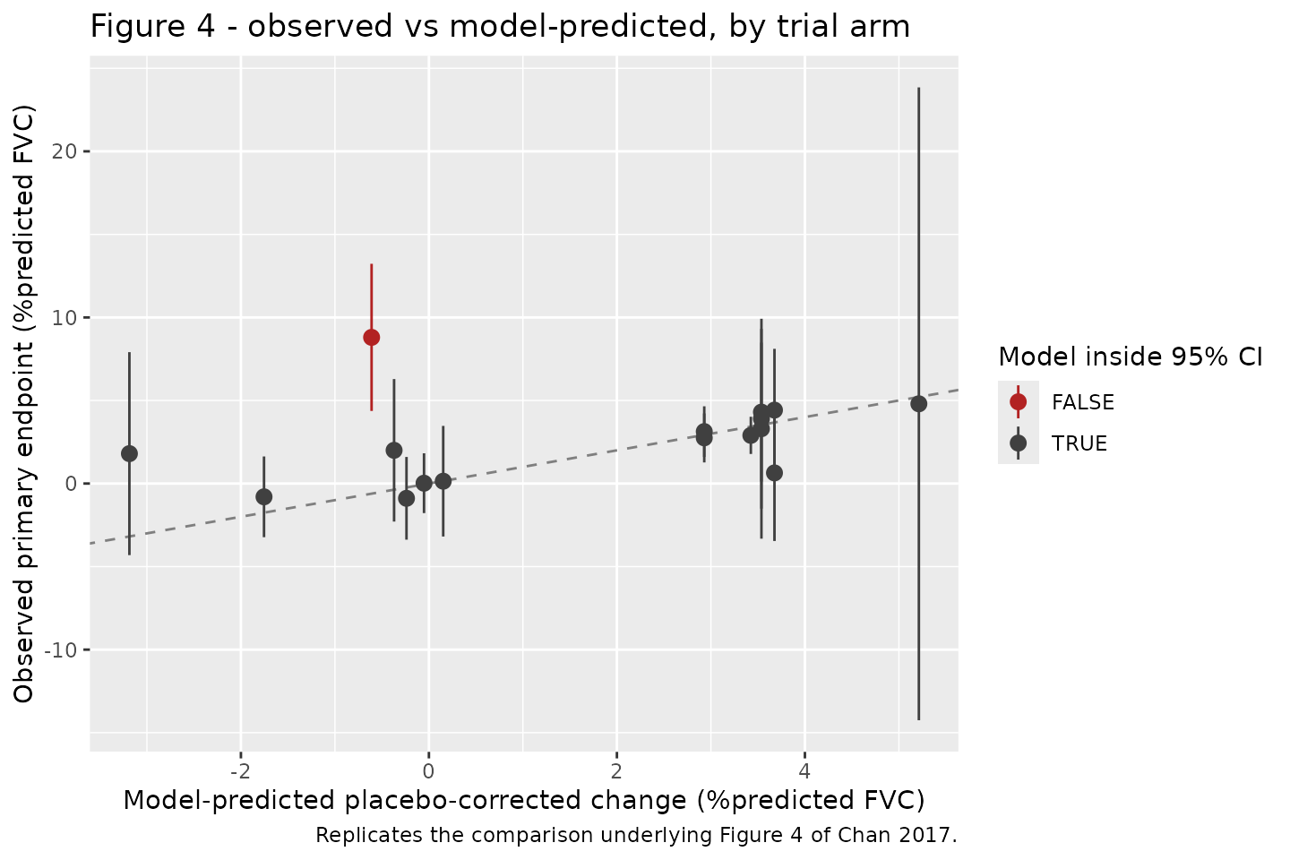
# Deterministic: no simulation noise, so the covered set is exact. 15 of 16
# arms are covered. The single miss is antoniou 2006, one of the four
# interferon-gamma trials that Chan 2017's Discussion itself singles out:
# "An obvious outlier is interferon gamma, of which two trials reported a large
# positive treatment effect, and two trials reported no treatment effect."
# The gate asserts both the count and that the miss is an interferon-gamma arm,
# so a regression that broke a different treatment would go red.
stopifnot(
  sum(cmp4$covered) == 15L,
  all(cmp4$treatment[!cmp4$covered] == "Interferon gamma")
)
Between-trial-arm variability
Chan 2017 Table 2 reports the between-trial-arm variability as
1.07 x 10^-6, with the note that its standard error “was
not estimated”. The model carries it, but it is numerically inert.
rxode2::rxSetSeed(20170907)

ev_eta <- build_arm(tgrid = 52, indicator = "NINTEDANIB", dose_high = 0L,
                    fvc_pctpred = 74, label = "Nintedanib")
ev_eta$id <- NULL

sim_eta <- rxode2::rxSolve(mod_full, events = ev_eta, nSub = 200,
                           omega = NULL) |>
  as.data.frame()

eta_sd <- stats::sd(sim_eta$fvcppcfb)

tibble::tibble(
  Quantity = c("Typical nintedanib effect at week 52 (%predicted FVC)",
               "SD across 200 simulated arms (%predicted FVC)",
               "SD implied by Table 2 read as a variance"),
  Value = c(mean(sim_eta$fvcppcfb), eta_sd, sqrt(1.07e-6))
) |>
  knitr::kable(digits = 6,
caption = "The between-arm random effect is three orders of magnitude below the effect it perturbs.")| Quantity | Value |
|---|---|
| Typical nintedanib effect at week 52 (%predicted FVC) | 2.929112 |
| SD across 200 simulated arms (%predicted FVC) | 0.001062 |
| SD implied by Table 2 read as a variance | 0.001034 |
# Wide headroom on purpose: the point is that the arm-level spread is
# negligible, not that it takes a particular value. sqrt(1.07e-6) = 0.00103,
# so 0.01 leaves an order of magnitude and still goes red if the variance were
# ever mis-scaled upward by 100x.
stopifnot(eta_sd < 0.01)
Why there is no PKNCA section
PKNCA validation does not apply here. This model has no drug
concentration, no dose events and no ODE states: it is an algebraic
regression of an arm-level efficacy endpoint on trial time. Cmax, Tmax,
AUC and half-life are undefined for it. The figure replications and
closed-form gates above are the validation, in the same way as for the
sibling algebraic MBMA vignettes
(Mercier_2014_tramadol_tapentadol,
Boucher_2018_naproxen_mbma).
Assumptions and deviations
Errata – the paper conflicts with itself on embase
Chan 2017 reports the baseline-%predicted-FVC covariate coefficient twice, with different values:
- Table 2, row “Baseline FVC effect (embase)”: 1.48 (95% CI -2.7 to 5.66).
- Results, covariate paragraph: 3.86 (95% CI -0.631 to 8.35).
Both are internally well formed – each point estimate sits at the centre of its own interval – so the confidence intervals cannot adjudicate. This model uses 1.48, on the following evidence, all of it internal to the paper:
- Table 2 is captioned “Parameter estimates of the final model”; the Results paragraph describes the covariate search.
-
Figure 5 plots the same treatments at two
baselines, so the ratio between its curves is
(76/67)^embasewith everything else cancelling. The figure reads about 1.25 (nintedanib) and 1.23 (pirfenidone);embase = 1.48predicts 1.21 andembase = 3.86predicts 1.63. Gated above. - Figure 5’s absolute levels agree with 1.48 too, including its 95% prediction interval: the dotted nintedanib band at week 52 reads about 2.0 to 4.05, and scaling the published Emax CI (2.15 to 4.47) the same way gives 1.98 to 4.12.
- Figure 3 confirms it independently at a different baseline (76.2): the week-24 pirfenidone 2,403 mg/day gap reads 2.55 and the model gives 2.555. Gated above.
The 3.86 value is therefore treated as an error in the Results text.
A reader who needs the alternative can refit with
ini(e_fvc_pctpred_emax = 3.86); note that doing so breaks
both figure gates.
Other assumptions and source notes
-
The placebo component is not reproducible. Chan
2017 estimated
E0_itnonparametrically (one free value per trial per timepoint) and did not tabulate it, so the model produces the placebo-corrected contrast only. This is a property of the source, not a simplification made here. See the scope table near the top. -
The residual is a unit-weight scale. Chan 2017 Eq.
1 defines the within-arm residual as normally distributed “with a
variance dependent on the sample size and observed SD of the trial arm”,
and used the inverse of that variance as the study weight. No sigma is
tabulated, because the weight is a property of each published arm rather
than of the model.
addSdis thereforefixed(1), following every other MBMA in this library. A bare stochasticrxSolve()will apply a 1.0 %predicted-FVC additive residual to every observation, which is the wrong magnitude for every arm in the dataset – too small for a 12-subject arm and too large for a 550-subject one. The operative per-observation SD is the arm’s own SD divided bysqrt(N_ARM). Every figure above usesrxode2::zeroRe(). -
The between-arm variance scale is unstated. Table
2’s
1.07e-6is not labelled as a variance or an SD, and its SE “was not estimated”. It is encoded as a variance per the nlmixr2~convention. The two readings differ by three orders of magnitude on a quantity that is already three to six orders below the effects it perturbs, so the choice has no practical consequence – as the gate above shows. -
Figure 5 baselines: 66/76 or 67/76? The Results
text says the simulation used “the observed medians (66% and 76%)” of
the stratified low and high baseline groups; the Figure 5 legend says
FVC=67andFVC=76. This vignette uses the figure’s own 67, since the figure is what is being replicated. Atembase = 1.48the difference between 66 and 67 moves the low-baseline curve by about 2%, well inside the digitisation tolerance. - Two dose discrepancies between Table 1 and Figure 4. Table 1 lists azathioprine as “3 mg” where Figure 4’s forest plot gives “3 mg/kg” (the clinically standard dosing, and almost certainly what Table 1 abbreviates), and colchicine as “1 mg” where Figure 4 gives the Douglas 1998 arm as “0.9 mg”. Neither affects any prediction: no dose enters the model, which identifies treatments by indicator only. Similarly, Figure 4 labels the two INPULSIS nintedanib arms 281.7 and 280.5 mg/day – exposure-weighted mean daily doses – against Table 1’s nominal 300 mg/day.
- The Figure 4 comparison uses the median baseline. Chan 2017 Figure 4 does not report per-trial baseline %predicted FVC, so the predictions in that section are computed at the dataset median of 74%. Arms whose true baseline departs from the median will be displaced by the covariate factor; the CAPACITY-2 and TOMORROW arms, whose baselines the paper does annotate (76.2 and 74.2), are handled at their own baselines in the Figure 3 section.
-
PRM-151 pools three dose levels. Chan 2017
attempted a dose-response for the 1, 5 and 10 mg/kg arms but reports
that it “resulted in minimization failures”, so a single Emax covers all
three. The model reproduces that: the
PRM151indicator carries no dose companion, and the three Figure 4 rows above therefore share one prediction. - Colchicine and prednisone are indirectly estimated. Neither had placebo-controlled IPF data; both reach placebo only through small active-control trials against interferon gamma (Chan 2017 Discussion). Their large negative point estimates and wide intervals should be read with that in mind, and simulations using them inherit the same indirection.
- Digitised reference values. The comparison columns in the Figure 3 and Figure 5 sections were read off the published panels rendered at 250-300 dpi, because neither figure carries numeric annotations. Reading precision is roughly +/- 0.1 %predicted FVC and the gates are set to 0.35 accordingly. Every other number in this vignette is a printed value from Table 1, Table 2, Figure 2 or Figure 4.