Inhalation PBPK with a partial-differential-equation lung (Boger 2018)
Source:vignettes/articles/Boger_2018_inhaled_pbpk.Rmd
Boger_2018_inhaled_pbpk.RmdBoger E, Wigstrom O. A Partial Differential Equation Approach to Inhalation Physiologically Based Pharmacokinetic Modeling. CPT Pharmacometrics Syst Pharmacol. 2018;7(10):638-646. doi:10.1002/psp4.12344.
This paper presents the first inhalation PBPK model that treats the lung as a continuous heterogeneous organ and the inhaled powder as a distribution that is continuous in both lung depth and particle size. The authors deposited their complete MATLAB implementation as Appendix S2, so every constant and every equation used here comes from a published source: the main text (Eqs 1-9, Tables 1-2), Appendix S1 (Eqs S1-S41, Tables S1-S3) or the deposited code.
There is no drug. The compound is a hypothetical neutral small molecule (MW 250 g/mol) relying on transcellular transport, used to demonstrate the framework in three case studies.
Model structure
Four processes act on the inhaled powder, and the model resolves all
of them along lung depth x:
- Deposition places particles along the airway tree as a function of particle size (typical-path Findeisen-Landahl model over a Weibel tree, with Cheng extrathoracic deposition; Eqs S24-S41).
- Dissolution shrinks each particle by the Nernst-Brunner equation into the epithelial lining fluid (ELF) of the slab it occupies (Eq. 3, recast as the non-singular squared-radius form of Eq. 10).
-
Mucociliary clearance (MCC) sweeps undissolved
particles proximally at a velocity proportional to the airway
cross-section (Eqs 2, S7) and delivers them to the gut (Eq. 5), where a
fraction
Fis absorbed. - Permeation carries dissolved drug ELF -> epithelium -> sub-epithelium -> blood, and back (Eqs 7-9), into a seven-tissue whole-body PBPK model (Eqs S8-S16).
Discretisation adopted here
rxode2 solves ODEs, so the two continuous coordinates are discretised by the method of lines, exactly as the authors do (Eq. S17):
| coordinate | states | count |
|---|---|---|
lung depth, tracheobronchial (x in [0, 2.2554] dm) |
elf_tb_slab<n>,
epithelium_tb_slab<n>,
subepithelium_tb_slab<n>
|
12 slabs |
lung depth, alveolar (x in [2.2554, 2.3290] dm) |
elf_alv_slab<n>,
epithelium_alv_slab<n>,
subepithelium_alv_slab<n>
|
8 slabs |
| particle size |
particles_<region>_<class>_slab<n>
(number density) and
pmass_<region>_<class>_slab<n> (z-moment,
z = r^2) |
8 size classes |
| whole body |
a_spleen, a_rapidly_perfused,
a_slowly_perfused, a_fat,
a_liver, a_gut, a_arterial,
a_venous, depot
|
9 |
that is, 9 systemic states, 3 * (12 + 8) = 60 lung
tissue states and 2 * 8 * (12 + 8) = 320 particle states:
389 ODEs in total.
The particle phase carries two conserved moments per (slab,
size class) rather than the authors’ shared-shrinkage variable.
That choice is what makes the discretised mass balance close: the number
density and the z-moment advect with the same conservative upwind MCC
operator, and the dissolution sink enters pmass_* and the
paired elf_* slab with identical magnitude and opposite
sign. The authors instead pre-integrate the MCC characteristics and
interpolate a two-dimensional table inside the right-hand side (Eqs
11-15), which rxode2 cannot express; the formulation used here is
mathematically the same Eq. 1 system, solved Eulerian in x
instead of by characteristics.
Population
str(mod$meta$population)
#> List of 3
#>  $ species   : chr "human"
#>  $ n_subjects: num 0
#>  $ notes     : chr "No subjects: a theoretical modelling exercise, not a fit to data. System physiology is a single 70 kg reference"| __truncated__
A single 70 kg reference adult; no subjects were fitted. Tissue volumes and blood flows are fractions of body weight and cardiac output from Table S1 (Brown et al.; Bernareggi and Rowland for the blood volumes), with a cardiac output of 5.2 L/min. The airway tree is Weibel geometry scaled to a functional residual capacity of 3,000 mL (Table S3); ELF, epithelial and sub-epithelial layer heights are from Table S2. Deposition assumes tidal breathing with a 1,000 mL tidal volume, 15 breaths/min, a 1:1 inspiratory:expiratory ratio and no breath hold.
Source trace
| Model element | Source |
|---|---|
lcl, bp, fup,
fuelf, lka, kpulung, MW,
density |
Table 2 (drug-specific parameters) |
peff |
Table 2 P_app = 1.5e-6 cm/s, converted to effective
permeability by the Sjogren 2013 relation implemented in Appendix S2
+drug/CalcPeffFromPapp.m
|
vdiff |
Table 2 v_diff = 8.5e-6 cm^2/s (Stokes-Einstein, MW
250) |
kpspleen … kpgut
|
Table 2, recomputed at full precision by Appendix S2
+drug/GetUpdatedKpValues_human.m (Rodgers/Simcyp values
rescaled so Vss = 140 L) |
foral |
Appendix S2 +drug/loadData.m
(data.F = 0.05); Table 2 prints F = 0.20 - see
Errata |
cs, rmu, rsd, lung-deposited
dose |
Table 1 and the case-study definitions in Results |
mccvel |
Eq. 2, alpha_0 = 3.6 mm/min (Yeates 1975) |
| tissue volumes / blood flows | Table S1 fractions x 70 kg / x 5.2 L/min |
airway N, D, L, angles |
Table S3 (Weibel, scaled to FRC 3,000 mL) |
| ELF / epithelium / sub-epithelium heights | Table S2 |
alveolar surface-area correction, f_al(x)
|
Eqs S18-S20; S_litt = 14,300 dm^2 |
cross-sectional areas A_f, A_ep,
A_sub
|
Eqs S21-S23 |
regional blood flows Q_br(x), Q_CO(x)
|
Eqs S4-S6 |
| MCC velocity profile | Eq. S7 |
| ELF / epithelium / sub-epithelium ODEs | Eqs 7-9 |
| whole-body PBPK ODEs | Eqs S8-S16 |
| particle transport / dissolution | Eqs 1, 3, 5, 10; discretised per Eq. S17 |
| deposition model | Eqs S24-S41 (reimplemented below) |
Regional deposition (Appendix S1 Eqs S24-S41)
The initial particle field is not part of the ODE system - it is the
initial condition. It is computed here by a direct R reimplementation of
Appendix S2’s +deposition package, whose equations are
printed as Eqs S24-S41.
Physiology tables
lung: Table S3 airway structure (lengths and diameters
in dm), Table S2 layer heights, and the Eq. S20 alveolarisation
fractions. x is the cumulative mid-airway depth,
cumsum(L) - L/2.
lung <- data.frame(
  gen = 1:24,
  L = c(1.026, .407, .1624, .065, .1086, .0915, .0769, .065, .0547, .0462,
        .0393, .0333, .0282, .0231, .0197, .0171, .0141, .0121, .01, .0085,
        .0071, .006, .005, .0043),
  D = c(.1539, .1043, .071, .0479, .0385, .0299, .0239, .0197, .0159, .0132,
        .0111, .0093, .0081, .007, .0063, .0056, .0051, .0046, .0043, .004,
        .0038, .0037, .0035, .0035),
  N = 2^(0:23),
  phi = c(20, 31, 43, 39, 39, 40, 36, 39, 45, 43, 45, 45, 60, 60, 60, 60,
          60, 60, 60, 60, 60, 60, 60, 60) * pi / 180,
  theta = c(95.5, 55.9, 32.8, 19.4, 40.4, 43.8, 46, 47.3, 49.3, 50.2, 50.7,
            51.3, 49.8, 47.2, 44.5, 43.4, 39.4, 45, 45, 45, 45, 45, 45, 45) * pi / 180,
  alv_frac = c(rep(0, 17), .002, .007, .02, .07, .139, .282, .48),
  h_tb = c(rep(1.1e-4, 9), rep(6e-5, 15)),
  h_al = rep(7e-7, 24)
)
lung$x <- cumsum(lung$L) - lung$L / 2
al_ind <- 16   # generations 1-16 tracheobronchial, 17-24 alveolar
Q_co <- 312    # L/h (5.2 L/min, Table S1)
BW <- 70
stopifnot(
  # The depth grid derived from Table S3 must reproduce the one in the
  # deposited +phys/lung_weibel.csv, including the tracheobronchial /
  # alveolar boundary at generation 16.
  abs(lung$x[al_ind] - 2.25545) < 1e-5,
  abs(lung$x[24] - 2.32895) < 1e-5,
  # Bare cylinder volume of the Weibel tree; the remaining 2,002 mL of the
  # 3,000 mL FRC is alveolar and is distributed by Eq. S20.
  abs(sum(lung$L * lung$N * pi * (lung$D / 2)^2) * 1000 - 997.86) < 0.1
)
Deposition equations
trapz_w <- function(x) {
  d <- diff(x)
  c(d[1] / 2, (head(d, -1) + tail(d, -1)) / 2, tail(d, 1) / 2)
}

# MATLAB's shape-preserving pchip, used by the deposited code wherever it
# interpolates a per-generation quantity onto the slab grid. Reimplemented
# rather than swapped for splinefun() so the initial particle field matches
# the one baked into the model file as its default.
pchip <- function(x, y, xi) {
  n <- length(x); h <- diff(x); del <- diff(y) / h; d <- numeric(n)
  k <- which(sign(del[-1]) * sign(del[-(n - 1)]) > 0)
  if (length(k)) {
    hs <- h[k] + h[k + 1]
    w1 <- (h[k] + hs) / (3 * hs); w2 <- (hs + h[k + 1]) / (3 * hs)
    dmax <- pmax(abs(del[k]), abs(del[k + 1]))
    dmin <- pmin(abs(del[k]), abs(del[k + 1]))
    d[k + 1] <- dmin / (w1 * (del[k] / dmax) + w2 * (del[k + 1] / dmax))
  }
  ends <- function(h1, h2, d1, d2) {
    dd <- ((2 * h1 + h2) * d1 - h1 * d2) / (h1 + h2)
    if (sign(dd) != sign(d1)) 0
    else if (sign(d1) != sign(d2) && abs(dd) > abs(3 * d1)) 3 * d1
    else dd
  }
  d[1] <- ends(h[1], h[2], del[1], del[2])
  d[n] <- ends(h[n - 1], h[n - 2], del[n - 1], del[n - 2])
  i <- findInterval(xi, x, all.inside = TRUE)
  hh <- x[i + 1] - x[i]; s <- xi - x[i]
  c3 <- (d[i] + d[i + 1] - 2 * (y[i + 1] - y[i]) / hh) / hh^2
  c2 <- ((y[i + 1] - y[i]) / hh - d[i]) / hh - c3 * hh
  y[i] + s * (d[i] + s * (c2 + s * c3))
}

# Eqs S24-S35: single-particle deposition physics.
part_params <- function(da_um) {
  da <- da_um * 1e-6
  kB <- 1.38064852e-23; Tk <- 273.15 + 37.5; eta <- 1.9224364e-5
  g <- 9.81; rho_a <- 1.1372; lam <- 0.066e-6
  Cd <- 1 + (lam / da) * (2.514 + 0.8 * exp(-0.55 * (da / lam)))
  list(Cd = Cd, eta = eta, rho_a = rho_a,
       vg = 1000 * ((da^2) * g * Cd) / (18 * eta),              # Eq. S29
       Dmol = (kB * Tk * Cd) / (3 * pi * eta * da))             # Eq. S34
}

# Eq. S24 (Cheng 2003 extrathoracic deposition). Q in cm^3/s, Dmol in m^2/s.
oral_dep <- function(Q, da_um, Dmol) {
  Qe <- Q * 60 / 1000
  1 - exp(-0.000278 * Qe * da_um^2 - 20.4 * (10000 * Dmol)^0.66 * Qe^-0.31)
}

# Eqs S25-S33 for one breathing phase; returns the per-generation, per-size
# deposition probability P_i of Eq. S36.
phase_prob <- function(da_um, D_cm, L_cm, N, V_scaled, Q, pp) {
  da <- da_um * 1e-6; D <- D_cm * 1e-2; L <- L_cm * 1e-2
  Qi <- Q / N
  v <- (Qi / (pi * (D_cm / 2)^2)) / 100                          # m/s
  ti <- V_scaled / N / Qi; ti[1] <- 0                            # s
  ng <- length(D); np <- length(da)
  IMP <- SED <- DIF <- matrix(0, ng, np)
  for (j in seq_len(np)) {
    stk <- 1000 * (da[j]^2) * v * pp$Cd[j] / (9 * pp$eta * D)    # Eq. S26
    IMP[, j] <- 0.768 * (L / (4 * D)) * stk                      # Eq. S25
    re <- pp$rho_a * D * v / pp$eta
    eps <- 3 * pp$vg[j] * ti * cos(pi / 4) / (4 * D)             # Eq. S28
    for (i in 2:ng) {
      e <- eps[i]
      # Eq. S27. MATLAB evaluates this in complex arithmetic and takes
      # real(); for eps >= 1 that collapses to complete sedimentation.
      SED[i, j] <- if (e >= 1) 1 else {
        s <- sqrt(1 - e^(2 / 3))
        2 / pi * (2 * e * s - (e^(1 / 3)) * s + asin(e^(1 / 3)))
      }
      sg <- pp$Dmol[j] * L[i] / (v[i] * D[i]^2)                  # Eq. S33
      DIF[i, j] <- if (re[i] > 2000) {                           # Eq. S32
        4 * sqrt(sg) * (1 - 0.444 * sqrt(sg))
      } else {
        1 - 0.819 * exp(-14.63 * sg) - 0.0976 * exp(-89.22 * sg) -
          0.0325 * exp(-228 * sg) - 0.0509 * exp(-125.9 * sg^(2 / 3))
      }
    }
  }
  IMP[1, ] <- oral_dep(Q, da_um, pp$Dmol)   # oral impaction replaces row 1
  1 - (1 - IMP) * (1 - SED) * (1 - DIF)     # Eq. S36
}

# Bolus scaling of Bondesson 2005, as implemented in +deposition/BolusScaling.m.
bolus_scale <- function(V, V_T = 1000, V_B = 1000, FRC = 3000) {
  Vi <- V * FRC / sum(V); n <- length(Vi); cV <- cumsum(Vi)
  scale_f <- sum(Vi) / (sum(Vi) - c(0, cV[-n]))
  scale_t <- vapply(seq_len(n), function(i) {
    (sum(Vi) + V_B) / sum(Vi[if (i == n) i:n else (i + 1):n])
  }, 0)
  chk <- V_T < ((cV[-n] + V_B) / (1 - cV[-n] / sum(Vi)))
  i_wash <- if (any(chk)) which.max(chk) else 1L
  if (all(!chk) == FALSE && i_wash == 1L) i_wash <- n
  scale_t[i_wash:n] <- (sum(Vi) + V_T) / sum(Vi)
  f_ave <- (scale_f + scale_t) / 2
  Vs <- f_ave * Vi; cVs <- cumsum(Vs)
  tst <- V_T < cVs[-n]
  imax <- if (any(tst)) which.max(tst) else n
  Vs[imax] <- V_T - cVs[imax - 1]
  if (imax < n) Vs[(imax + 1):n] <- Vi[(imax + 1):n]
  cVs <- cumsum(Vs)
  fb <- numeric(n); if (i_wash > 1) fb[seq_len(i_wash - 1)] <- 1
  vf <- numeric(n)
  for (i in i_wash:imax) vf[i] <- (V_T - cVs[i - 1]) / V_B
  fb[i_wash:imax] <- pmin(1, vf[i_wash:imax])
  fp <- numeric(n)
  for (i in 2:imax) fp[i] <- if (i < imax) fb[i] - fb[i + 1] else 1 - sum(fp)
  list(f_ave = f_ave, V = Vs, imax = imax, frac_bolus = fb, frac_pause = fp)
}
# Prepend a row for the extrathoracic region (Eqs S37-S41 index it as i = 1).
N <- c(0, lung$N); Lcm <- c(0, lung$L) * 10; Dcm <- c(0, lung$D) * 10
V <- Lcm * N * pi * (Dcm / 2)^2
V <- V + c(0, lung$alv_frac) * (3000 - sum(V))
bs <- bolus_scale(V)
Lsc <- Lcm * bs$f_ave^(1 / 3); Dsc <- Dcm * bs$f_ave^(1 / 3)

da_grid <- 10^seq(log10(0.00015), log10(20), length.out = 1000)   # um, as in +deposition/Deposition.m
pp <- part_params(da_grid)
P_in <- phase_prob(da_grid, Dsc, Lsc, N, bs$V, 1000 / (0.5 / 15) / 60, pp)
P_ex <- phase_prob(da_grid, Dsc, Lsc, N, bs$V, 1000 / (0.5 / 15) / 60, pp)

# Eqs S37-S41 with zero breath-hold time (Table S3 breathing pattern).
ng <- bs$imax; np <- length(da_grid)
Ph <- rbind(0, P_in[seq_len(ng), , drop = FALSE])
fmat <- t(vapply(seq_len(ng + 1), function(i) apply(1 - Ph[seq_len(i), , drop = FALSE], 2, prod), numeric(np)))
beta <- fmat[3:(ng + 1), , drop = FALSE] * bs$frac_pause[2:ng]
xmat <- matrix(0, ng, np)
for (i in (ng - 1):1) xmat[i, ] <- (1 - P_ex[i + 1, ]) * xmat[i + 1, ] + beta[i, ]
df_dep <- fmat[seq_len(ng), , drop = FALSE] * P_in[seq_len(ng), , drop = FALSE] * bs$frac_bolus[seq_len(ng)] +
  xmat * P_ex[seq_len(ng), , drop = FALSE]
df_dep <- rbind(df_dep, matrix(0, length(N) - nrow(df_dep), np))
Gate 1: published extrathoracic deposition fractions
The paper states (Results, case study 2) that extrathoracic deposition is 1.0%, 3.3% and 10.1% for the small, medium and large particle size distributions. Those three printed numbers are the only quantitative check the paper offers on the deposition model, and they are reproduced here from the Eqs S24-S41 reimplementation alone.
psd <- list(small = c(0.75, 0.15), medium = c(1.5, 0.3), large = c(3, 0.6))  # diameter mean, sd (um)

# The particle radius grid is the aerodynamic diameter grid halved: the
# compound's density is 1 g/cm^3 and the shape factor is 1, so aerodynamic and
# geometric diameter coincide (+deposition/Deposition.m, `da_to_d`).
r_um <- da_grid / 2

et_fraction <- function(mu_d, sd_d) {
  y <- dnorm(r_um, mu_d / 2, sd_d / 2)     # mass density over radius
  ydep <- sweep(df_dep, 2, y, `*`)
  w <- trapz_w(r_um)
  c(ET = sum(ydep[1, ] * w), lung = sum(as.vector(ydep[-1, , drop = FALSE] %*% w)))
}
et <- vapply(psd, function(p) et_fraction(p[1], p[2]), numeric(2))
gate1 <- data.frame(
  PSD = names(psd),
  `Simulated ET deposition (%)` = round(100 * et["ET", ], 2),
  `Published ET deposition (%)` = c(1.0, 3.3, 10.1),
  check.names = FALSE
)
knitr::kable(gate1, row.names = FALSE)| PSD | Simulated ET deposition (%) | Published ET deposition (%) |
|---|---|---|
| small | 0.98 | 1.0 |
| medium | 3.21 | 3.3 |
| large | 9.43 | 10.1 |
Building the initial particle field
p0(x, r) is the deposited number of particles per unit
radius per unit lung depth. It is binned onto the model’s
K = 8 equal-width radius classes, integrating in
z = r^2 because that is the measure the paper’s mass
expression (Eq. S1) uses, and then rescaled so the discretised particle
mass equals the lung-deposited dose exactly.
NU <- 12; NL <- 8; KB <- 8; LET <- letters[1:KB]
dens <- 4e9        # nmol/dm^3 (rho = 1 g/cm^3, MW = 250 g/mol)
MW <- 250
xb <- c(0, lung$x[al_ind], lung$x[24])
x_u <- seq(xb[1], xb[2], length.out = NU); dx_u <- trapz_w(x_u)
x_l <- seq(xb[2], xb[3], length.out = NL); dx_l <- trapz_w(x_l)

particle_field <- function(mu_d, sd_d, ldd_ug) {
  mu <- mu_d / 2 * 1e-5; sg <- sd_d / 2 * 1e-5     # radius mean / sd, dm
  r <- r_um * 1e-5                                  # radius grid, dm
  y <- dnorm(r, mu, sg)
  ydep <- sweep(df_dep, 2, y, `*`)
  w <- trapz_w(r)
  ymd <- ydep / sum(as.vector(ydep %*% w)) * ldd_ug * 1e-6      # g per unit radius
  mp <- r^3 * 4 * pi / 3 * 1000                                 # g per particle
  npart <- sweep(ymd[-1, , drop = FALSE], 2, mp, `/`) / lung$L  # number per unit radius per unit depth

  bin <- function(xg) {
    # rows = slabs on xg, columns = the fine radius grid
    p0 <- apply(npart, 2, function(col) pchip(lung$x, col, xg))
    hr <- 7 * sg / KB
    ctr <- mu + (seq_len(KB) - (KB + 1) / 2) * hr
    n <- matrix(0, length(xg), KB)
    for (j in seq_len(KB)) {
      rr <- seq(ctr[j] - hr / 2, ctr[j] + hr / 2, length.out = 41)
      Y <- apply(p0, 1, function(row) approx(r, row, rr, rule = 2)$y)
      n[, j] <- as.vector(t(Y) %*% (trapz_w(rr) * 2 * rr))       # dz = 2 r dr
    }
    list(n = n, z = ctr^2)
  }
  bu <- bin(x_u); bl <- bin(x_l)
  mass <- dens * 2 / 3 * pi * (sum(dx_u * (bu$n %*% bu$z)) + sum(dx_l * (bl$n %*% bl$z)))
  s <- (ldd_ug * 1e-6 / MW * 1e9) / mass
  ET_df <- sum(ydep[1, ] * w)
  lung_df <- sum(as.vector(ydep[-1, , drop = FALSE] %*% w))
  list(nu = bu$n * s, nl = bl$n * s, z = bu$z, rmu = mu, rsd = sg,
       # Eq. S16 initial condition: the inhaled dose that deposited
       # extrathoracically and was swallowed.
       ET_nmol = (ldd_ug / lung_df * ET_df) * 1e-6 / MW * 1e9)
}

make_inits <- function(pf) {
  v <- c(depot = unname(pf$ET_nmol))
  for (k in seq_len(NU)) for (j in seq_len(KB)) {
    v[sprintf("particles_tb_%s_slab%d", LET[j], k)] <- pf$nu[k, j]
    v[sprintf("pmass_tb_%s_slab%d", LET[j], k)] <- pf$nu[k, j] * pf$z[j]
  }
  for (k in seq_len(NL)) for (j in seq_len(KB)) {
    v[sprintf("particles_alv_%s_slab%d", LET[j], k)] <- pf$nl[k, j]
    v[sprintf("pmass_alv_%s_slab%d", LET[j], k)] <- pf$nl[k, j] * pf$z[j]
  }
  v
}

simulate_case <- function(mu_d, sd_d, ldd_ug, cs, mcc = 2.16, tmax = 36) {
  pf <- particle_field(mu_d, sd_d, ldd_ug)
  s <- rxSolve(mod, et(seq(0, tmax, by = 0.25)),
    params = c(rmu = pf$rmu, rsd = pf$rsd, cs = cs, mccvel = mcc),
    inits = make_inits(pf), returnType = "data.frame", atol = 1e-10, rtol = 1e-8)
  s$ldd_ug <- ldd_ug
  s
}
Gate 3: systemic disposition reproduces the printed CL and Vss
Table 2 states a blood clearance of 70 L/h and a
steady-state volume of distribution of 140 L. Both are
properties of the whole-body PBPK half of the model alone, so an
intravenous bolus into venous blood - with no particles and no swallowed
dose - recovers them in closed form. This is a strict check:
AUC(0-inf) = Dose / CL holds exactly for a linear system,
and Vss follows from the mean residence time.
empty_particles <- setNames(
  rep(0, 2 * KB * (NU + NL)),
  c(outer(LET, seq_len(NU), function(a, k) sprintf("particles_tb_%s_slab%d", a, k)),
    outer(LET, seq_len(NU), function(a, k) sprintf("pmass_tb_%s_slab%d", a, k)),
    outer(LET, seq_len(NL), function(a, k) sprintf("particles_alv_%s_slab%d", a, k)),
    outer(LET, seq_len(NL), function(a, k) sprintf("pmass_alv_%s_slab%d", a, k))))

# The venous pool mixes with a time constant of V_venous / cardiac output =
# 3.6 / 312 = 0.012 h, so the first minutes have to be sampled densely or the
# trapezoidal AUC is badly biased on the steep distribution phase.
t_iv <- unique(c(0, 10^seq(-5, log10(0.5), length.out = 500),
                 seq(0.5, 5, by = 0.005), seq(5, 200, by = 0.05)))
iv <- rxSolve(mod, et(amt = 1000, cmt = "a_venous") %>% et(t_iv),
  inits = c(depot = 0, empty_particles),
  returnType = "data.frame", atol = 1e-12, rtol = 1e-10)

conc <- iv %>% filter(!is.na(Cc)) %>% mutate(id = 1L, treatment = "IV bolus")
o_conc <- PKNCAconc(conc, Cc ~ time | treatment + id, concu = "nM", timeu = "h")
o_dose <- PKNCAdose(data.frame(id = 1L, treatment = "IV bolus", time = 0, dose = 1000),
                    dose ~ time | treatment + id, doseu = "nmol")
res <- pk.nca(PKNCAdata(o_conc, o_dose,
  intervals = data.frame(start = 0, end = Inf, aucinf.obs = TRUE, cmax = TRUE,
                         half.life = TRUE, cl.obs = TRUE, vss.obs = TRUE),
  options = list(auc.method = "lin up/log down")))
nca <- as.data.frame(res) %>% select(PPTESTCD, PPORRES)

gate3 <- data.frame(
  `NCA parameter` = c("CL (L/h)", "Vss (L)"),
  Simulated = c(nca$PPORRES[nca$PPTESTCD == "cl.obs"], nca$PPORRES[nca$PPTESTCD == "vss.obs"]),
  `Table 2` = c(70, 140), check.names = FALSE
)
gate3$`Difference (%)` <- round(100 * (gate3$Simulated / gate3$`Table 2` - 1), 2)
knitr::kable(gate3, digits = 3)| NCA parameter | Simulated | Table 2 | Difference (%) |
|---|---|---|---|
| CL (L/h) | 69.999 | 70 | 0.00 |
| Vss (L) | 139.942 | 140 | -0.04 |
Gate 4: mass balance closes exactly
Switching off both elimination routes (cl = 0,
foral = 1) makes the system closed, so the sum over every
state must stay at the lung-deposited dose plus the swallowed
extrathoracic dose for all 36 hours. This is the check that the
conservative two-moment particle discretisation was introduced to
satisfy.
pf1 <- particle_field(3, 0.6, 100)
closed <- rxSolve(mod, et(seq(0, 36, by = 1)),
  params = c(rmu = pf1$rmu, rsd = pf1$rsd, cs = 100, mccvel = 2.16, lcl = -30, foral = 1),
  inits = make_inits(pf1), returnType = "data.frame", atol = 1e-12, rtol = 1e-10)

sys_states <- c("a_spleen", "a_rapidly_perfused", "a_slowly_perfused", "a_fat",
                "a_liver", "a_gut", "a_arterial", "a_venous", "depot")
total <- rowSums(closed[, sys_states]) + closed$alung
expected <- 100e-6 / MW * 1e9 + unname(pf1$ET_nmol)
range(total)
#> [1] 460.5744 460.5744
stopifnot(max(abs(total / expected - 1)) < 1e-6)
Case study 1: mucociliary clearance and particle size distribution
Table 1: C_s = 100 nM, lung-deposited dose 100 ug, wide
(large) PSD. Scenario (ii) replaces the PSD with a narrow one centred on
the same mass median diameter; scenario (iii) switches MCC off.
cs1 <- bind_rows(
  simulate_case(3, 0.6,  100, 100, mcc = 2.16) %>% mutate(scenario = "MCC + wide PSD"),
  simulate_case(3, 0.06, 100, 100, mcc = 2.16) %>% mutate(scenario = "MCC + narrow PSD"),
  simulate_case(3, 0.6,  100, 100, mcc = 0)    %>% mutate(scenario = "No MCC + wide PSD")
)
cs1_long <- cs1 %>%
  select(time, scenario, Lung = Clung, Plasma = Cc) %>%
  tidyr::pivot_longer(c(Lung, Plasma), names_to = "matrix", values_to = "conc") %>%
  filter(conc > 0)   # the log axis cannot show the t = 0 plasma zero

ggplot(cs1_long, aes(time, conc, colour = scenario, linetype = matrix)) +
  geom_line(linewidth = 0.7) +
  scale_y_log10(limits = c(1e-5, 1e5)) +
  scale_x_continuous(breaks = seq(0, 36, 6)) +
  scale_colour_manual(values = c("MCC + wide PSD" = "blue", "MCC + narrow PSD" = "red",
                                 "No MCC + wide PSD" = "black")) +
  labs(x = "Time (hours)", y = "Concentration (nM)", colour = NULL, linetype = NULL,
       title = "Replicates Figure 3a of Boger 2018")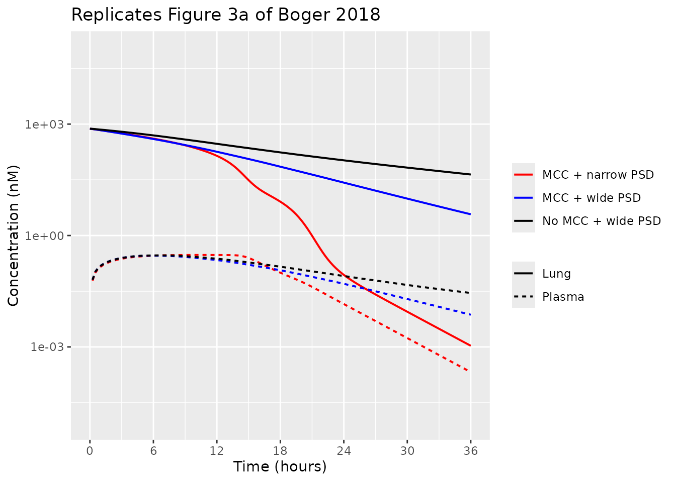
The paper’s three qualitative conclusions from this panel are that neglecting MCC makes lung retention erroneously long, that a narrow PSD dissolves more rapidly, giving an earlier and more distinct drop in lung concentrations, and that the plasma profile is far less affected than the lung profile.
c1 <- cs1 %>%
  mutate(scenario = factor(scenario, c("MCC + wide PSD", "MCC + narrow PSD", "No MCC + wide PSD"))) %>%
  group_by(scenario) %>%
  summarise(Cmax = max(Cc), Tmax = time[which.max(Cc)],
            lung_12h = Clung[time == 12], lung_36h = Clung[time == 36], .groups = "drop")
knitr::kable(c1, digits = c(0, 4, 2, 2, 4))| scenario | Cmax | Tmax | lung_12h | lung_36h |
|---|---|---|---|---|
| MCC + wide PSD | 0.2859 | 6.00 | 180.01 | 3.7277 |
| MCC + narrow PSD | 0.2994 | 10.25 | 139.83 | 0.0011 |
| No MCC + wide PSD | 0.2912 | 6.50 | 294.63 | 43.9455 |
stopifnot(
  # Switching MCC off leaves several-fold more drug in the lung at 36 h.
  c1$lung_36h[c1$scenario == "No MCC + wide PSD"] >
    3 * c1$lung_36h[c1$scenario == "MCC + wide PSD"],
  # The narrow PSD empties the lung far faster than the wide one.
  c1$lung_36h[c1$scenario == "MCC + narrow PSD"] <
    c1$lung_36h[c1$scenario == "MCC + wide PSD"],
  # Plasma Cmax is comparatively insensitive to all three scenarios.
  max(c1$Cmax) / min(c1$Cmax) < 1.5
)
Case study 2: particle size distribution
Table 1: C_s = 250 nM, lung-deposited dose 50 ug, three
PSDs.
cs2 <- bind_rows(lapply(names(psd), function(nm) {
  simulate_case(psd[[nm]][1], psd[[nm]][2], 50, 250) %>% mutate(PSD = nm)
})) %>% mutate(PSD = factor(PSD, names(psd)))

cs2 %>%
  select(time, PSD, Lung = Clung, Plasma = Cc) %>%
  tidyr::pivot_longer(c(Lung, Plasma), names_to = "matrix", values_to = "conc") %>%
  filter(conc > 0) %>%
  ggplot(aes(time, conc, colour = PSD, linetype = matrix)) +
  geom_line(linewidth = 0.7) +
  scale_y_log10(limits = c(1e-5, 1e5)) +
  scale_x_continuous(breaks = seq(0, 36, 6)) +
  scale_colour_manual(values = c(small = "blue", medium = "red", large = "black")) +
  labs(x = "Time (hours)", y = "Concentration (nM)", colour = "PSD", linetype = NULL,
       title = "Replicates Figure 3b of Boger 2018")
#> Warning: Removed 25 rows containing missing values or values outside the scale range
#> (`geom_line()`).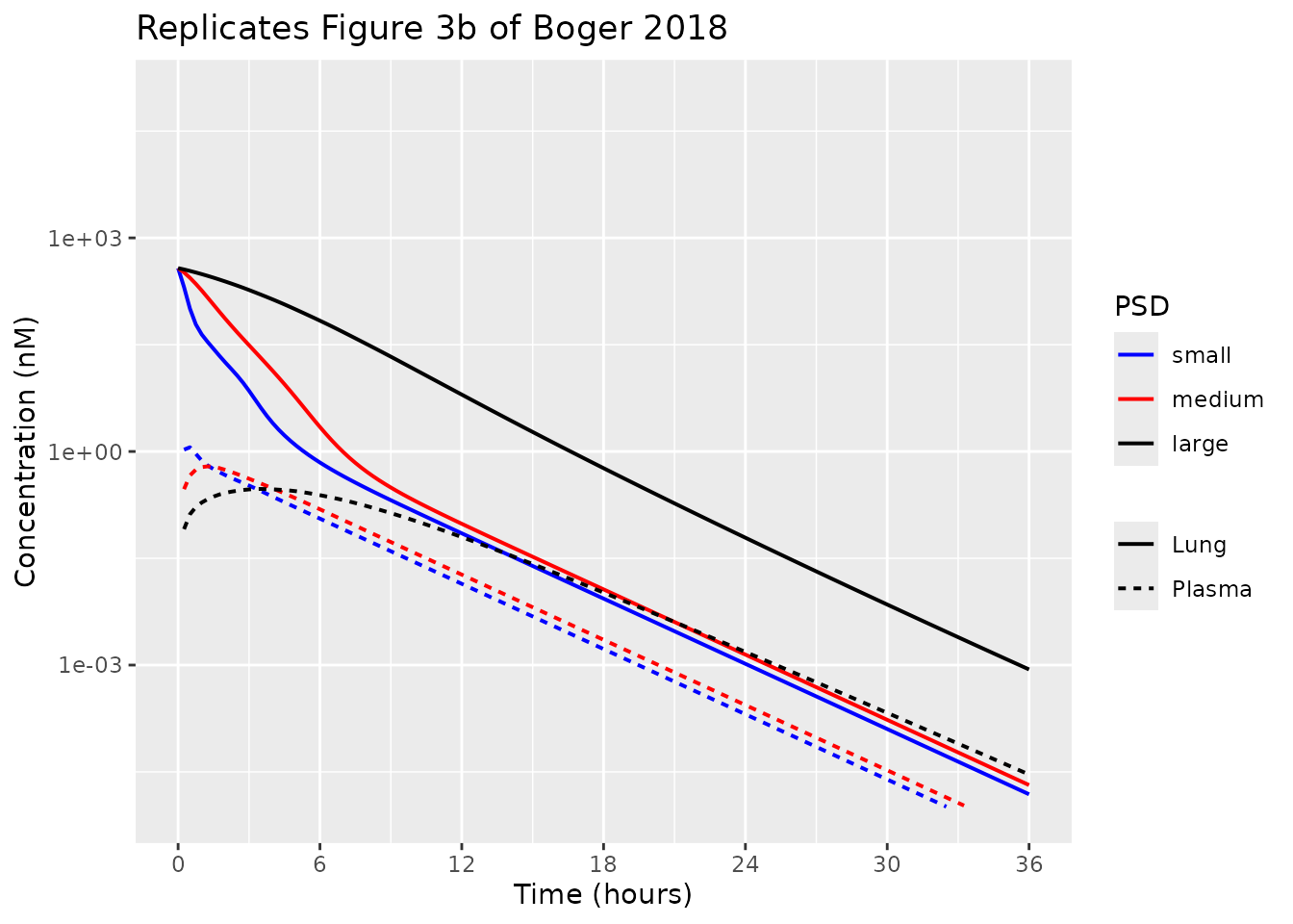
PKNCA summary of the simulated plasma profiles
conc2 <- cs2 %>% filter(!is.na(Cc)) %>% mutate(id = as.integer(PSD), treatment = as.character(PSD))
# Lung-deposited dose, 50 ug = 200 nmol at MW 250.
d2 <- conc2 %>% distinct(id, treatment) %>% mutate(time = 0, dose = 50e-6 / MW * 1e9)
res2 <- pk.nca(PKNCAdata(
  PKNCAconc(conc2, Cc ~ time | treatment + id, concu = "nM", timeu = "h"),
  PKNCAdose(d2, dose ~ time | treatment + id, doseu = "nmol"),
  intervals = data.frame(start = 0, end = 36, cmax = TRUE, tmax = TRUE,
                         auclast = TRUE, half.life = TRUE)))
nca2 <- as.data.frame(res2) %>%
  filter(PPTESTCD %in% c("cmax", "tmax", "auclast", "half.life")) %>%
  select(treatment, PPTESTCD, PPORRES) %>%
  tidyr::pivot_wider(names_from = PPTESTCD, values_from = PPORRES) %>%
  mutate(treatment = factor(treatment, names(psd))) %>%
  arrange(treatment) %>%
  rename("PSD" = treatment, "Cmax (nM)" = cmax, "Tmax (h)" = tmax,
         "AUC0-36 (nM*h)" = auclast, "t-half (h)" = half.life)
knitr::kable(nca2, digits = 3)| PSD | AUC0-36 (nM*h) | Cmax (nM) | Tmax (h) | t-half (h) |
|---|---|---|---|---|
| small | 2.783 | 1.146 | 0.50 | 1.968 |
| medium | 2.718 | 0.618 | 1.25 | 1.978 |
| large | 2.537 | 0.298 | 3.50 | 2.126 |
stopifnot(
  # The paper's headline result for this panel, reproducing Usmani 2014:
  # "smaller particles achieve a higher and earlier plasma peak".
  nca2$`Cmax (nM)`[1] > nca2$`Cmax (nM)`[2], nca2$`Cmax (nM)`[2] > nca2$`Cmax (nM)`[3],
  nca2$`Tmax (h)`[1] < nca2$`Tmax (h)`[2], nca2$`Tmax (h)`[2] < nca2$`Tmax (h)`[3]
)
The paper reports no NCA of its own, so there is no published table to compare against; the ordering assertions above are the quantitative form of the conclusion the authors draw from Figure 3b.
The paper also notes that larger PSDs deposit more in the extrathoracic region, quantified in Gate 1 above (1.0 / 3.3 / 10.1%).
Case study 3: overdosing
Table 1: C_s = 100 nM, wide PSD, lung-deposited doses of
100, 400 and 1,600 ug. The paper’s finding is a small
nonlinearity in dose-normalised plasma concentration, “particularly
pronounced at t > 24 hour”, alongside a marked loss of lung
targeting.
cs3 <- bind_rows(lapply(c(100, 400, 1600), function(d) {
  simulate_case(3, 0.6, d, 100) %>% mutate(LDD = factor(d, c(100, 400, 1600)))
}))

ggplot(filter(cs3, Cc > 0), aes(time, Cc / ldd_ug, colour = LDD)) +
  geom_line(linewidth = 0.7, linetype = "dashed") +
  scale_y_log10() + scale_x_continuous(breaks = seq(0, 36, 6)) +
  scale_colour_manual(values = c("100" = "blue", "400" = "red", "1600" = "black")) +
  labs(x = "Time (hours)", y = "Dose-normalised concentration",
       colour = "LDD (ug)", title = "Replicates Figure 3c of Boger 2018")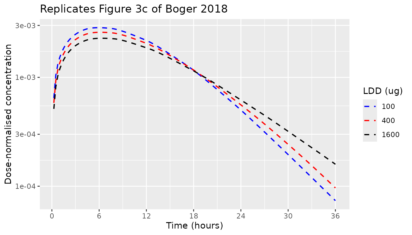
dn <- cs3 %>% group_by(LDD) %>%
  summarise(peak = max(Cc / ldd_ug), at6 = (Cc / ldd_ug)[time == 6],
            at36 = (Cc / ldd_ug)[time == 36], .groups = "drop")
knitr::kable(dn, digits = 6)| LDD | peak | at6 | at36 |
|---|---|---|---|
| 100 | 0.002859 | 0.002859 | 0.000074 |
| 400 | 0.002594 | 0.002593 | 0.000096 |
| 1600 | 0.002287 | 0.002285 | 0.000159 |
stopifnot(
  # Figure 3c: the dose-normalised curves are ordered 100 > 400 > 1600 early
  # and reverse by 36 h - a nonlinearity, but a small one.
  dn$at6[1] > dn$at6[2], dn$at6[2] > dn$at6[3],
  dn$at36[1] < dn$at36[2], dn$at36[2] < dn$at36[3],
  max(dn$peak) / min(dn$peak) < 1.5
)
Lung targeting
The paper defines lung targeting as the ratio of free concentration in a pulmonary sub-region to free plasma concentration, and reports that it markedly decreases with increasing dose and converges to 1 at long times (Figure 4g-i).
The epithelial slab volumes are fixed constants of the discretisation and are identical across the three arms, so the ratio of total tracheobronchial epithelial amount to free plasma concentration is proportional to the paper’s targeting metric with the same constant of proportionality in every arm. Expressing each arm relative to the 100 ug arm therefore cancels that constant and gives the dose effect the paper reports, without needing the slab volumes.
epi_slabs <- sprintf("epithelium_tb_slab%d", seq_len(NU))
tgt <- cs3 %>%
  mutate(free_plasma = 0.75 * Cc,
         free_epi = rowSums(across(all_of(epi_slabs)))) %>%
  group_by(LDD) %>%
  summarise(`1 h` = (free_epi / free_plasma)[time == 1],
            `6 h` = (free_epi / free_plasma)[time == 6],
            `36 h` = (free_epi / free_plasma)[time == 36], .groups = "drop")
tgt[, -1] <- sweep(as.matrix(tgt[, -1]), 2, as.numeric(tgt[1, -1]), `/`)
knitr::kable(tgt, digits = 3,
caption = "Relative lung targeting (100 ug arm = 1 at each time)")| LDD | 1 h | 6 h | 36 h |
|---|---|---|---|
| 100 | 1.000 | 1.000 | 1.000 |
| 400 | 0.641 | 0.733 | 1.749 |
| 1600 | 0.378 | 0.468 | 2.820 |
stopifnot(
  # Targeting falls monotonically with dose at every time point examined.
  tgt$`1 h`[1] >= tgt$`1 h`[2], tgt$`1 h`[2] >= tgt$`1 h`[3],
  tgt$`6 h`[1] >= tgt$`6 h`[2], tgt$`6 h`[2] >= tgt$`6 h`[3]
)
Grid convergence
The slab and size-class counts are numerical choices, not properties of the paper, so they have to be auditable. The table below was produced by regenerating the model at five discretisations and simulating case study 1 scenario (i); it is reproduced here rather than recomputed at render time because each row requires a different model file.
| N_tb | N_alv | K | ODEs | Cmax (nM) | AUC(0-36) | Clung(12 h) | solve (s) |
|---|---|---|---|---|---|---|---|
| 4 | 3 | 4 | 86 | 0.2673 | 4.851 | 258.7 | 1.5 |
| 6 | 4 | 5 | 139 | 0.2716 | 4.618 | 216.3 | 2.1 |
| 8 | 6 | 6 | 219 | 0.2879 | 4.710 | 199.2 | 3.5 |
| 12 | 8 | 8 | 389 | 0.2859 | 4.633 | 180.0 | 8.5 |
| 16 | 12 | 10 | 653 | 0.2899 | 4.617 | 169.6 | 24.8 |
Relative to the finest grid, the shipped 12 / 8 / 8
discretisation is within 1.4% on plasma Cmax,
0.3% on plasma AUC and 6.1% on lung
concentration at 12 h. The systemic endpoints - the ones the published
figures can be read against - are converged; the lung concentration
converges more slowly because each discrete size class dissolves at a
discrete time, which smooths the terminal lung profile. A user who needs
the lung profile at higher fidelity should regenerate at a finer
grid.
Assumptions and deviations
Errata and source conflicts
-
Oral bioavailability. Table 2 prints
F = 0.20; the deposited code (+drug/loadData.m) usesdata.F = 0.05, and that is the value used to produce the published figures. The code value is adopted, per the standing rule that a deposited implementation outranks the printed table. Settingforal = 0.2recovers the Table 2 reading. -
Eq. S15 (venous blood) is internally inconsistent.
As printed, it subtracts
Q_i * C_vefor every tissue, which would make venous blood perfuse the tissues in addition to the arterial supply already written in Eqs S8-S11; the resulting system does not conserve mass. It also routes the bronchial circulation from venous blood, whereas Figure 2 and the depositedCreateModel.mroute it from arterial blood, which is the physiologically correct source. The deposited code is followed. -
Eq. S17 sign. The printed forward-difference scheme
writes
d(delta_k)/dt = gamma + alpha(x_k) * (delta_{k+1} - delta_k)/(x_{k+1} - x_k). For the advection equationd(delta)/dt + alpha * d(delta)/dx = gammawith thealpha <= 0convention of Eq. S7, the advective term carries a minus sign, which is what the deposited code implements. The code is followed. -
Particle mass convention. The paper’s mass
expression (Eq. S1,
m = rho * (2/3) * pi * integral z * p dz) is exact only att = 0; once particles have shrunk bydelta,rho * (2/3) * pi * integral (z + delta) * p_0 dzis not identical torho * (4/3) * pi * integral r^3 p dr. The authors’ convention is nevertheless self-consistent - their mass-transfer rate (Eq. S2) is the exact derivative of their mass - so the model conserves mass within its own bookkeeping, and it is that bookkeeping that produced the published figures. It is reproduced unchanged here. -
Table 2 partition coefficients are rounded. Table 2
prints
Kpto two significant figures; the deposited+drug/GetUpdatedKpValues_human.mcomputes them from Rodgers/Simcyp values rescaled by a single factor so thatVss= 140 L exactly. The full-precision values are used, and they round to the printed ones (3.88 -> 3.9, 3.08 -> 3.1, 2.32 -> 2.3, 0.556 -> 0.56, 5.93 -> 5.9, 3.70 -> 3.7, 4.875 -> 4.9). - A stale comment in the deposited code describes the parameter set as “salbutamol in humans” and a second describes the partition coefficients as “rat Kp-values”. Neither is consistent with the manuscript, which never names a drug and describes the compound only as a neutral small molecule; the Table 2 values do not match salbutamol. The model is documented as a generic compound.
-
An extra factor of two on permeability.
+drug/loadData.msetsdata.P = 2 * data.P * data.scaleP. The manuscript describes only the ten-fold alveolar scaling (Appendix S1 section 1.2), not the factor of two. The code is followed, since it generated the published figures.
Numerical deviations from the authors’ implementation
-
Eulerian rather than characteristic particle
transport. The authors reduce the two-dimensional particle PDE
by pre-integrating the MCC characteristics (
x0,nu; Eqs 11-14) and interpolating a two-dimensional table of the initial distribution inside the ODE right-hand side (Eq. 15). rxode2 has no in-model interpolation, so the same Eq. 1 system is solved directly on a fixed(x, size-class)grid with two conserved moments per cell. This is a different numerical scheme for the same equations, not a different model; Gate 4 shows it conserves mass exactly. - Coarser grids. The paper uses 100 slabs per region and a continuous 1,000-point particle size distribution; this model uses 12 / 8 slabs and 8 size classes, with the convergence evidence tabulated above.
- Extrathoracic deposition reproduces to 0.98 / 3.21 / 9.43% against the published 1.0 / 3.3 / 10.1%. The residual comes from MATLAB-vs-R differences in the cubic interpolation used inside the Eqs S37-S41 exhalation cascade.
Assumptions
- The deposited MATLAB code is treated as authoritative wherever it conflicts with the printed equations, per the errata above. Every such conflict is listed; none was resolved silently.
- No inter-individual variability and no residual-error model are encoded, because the paper reports none: this is a deterministic forward-simulation model, not a fit to data.
- The particle size distribution is normal in radius with the
mean and standard deviation given as diameters in the paper, matching
the deposited
+deposition/Deposition.m, and it is interpreted as a mass density over radius (which is what makesy_depa mass in the deposited code, and is the usual convention for a mass median aerodynamic diameter). - Scenario inputs (particle size distribution, lung-deposited dose,
solubility, MCC on/off) are supplied through
rxSolve(params = , inits = ); the model file ships case study 1 scenario (i) as its default initial state.