One-compartment IV-bolus BQL methodology template (Beal 2001)
Source:vignettes/articles/Beal_2001_iv1cmt_bql.Rmd
Beal_2001_iv1cmt_bql.RmdModel and source
- Citation: Beal SL. Ways to fit a PK model with some data below the quantification limit. J Pharmacokinet Pharmacodyn. 2001 Oct;28(5):481-504. doi:10.1023/a:1012299115260. PMID 11768292.
- Description: Methodology reference. One-compartment IV-bolus generative toy model from Beal 2001 (the M1-M7 BQL methods paper). Typical CL is fixed at 0.693 and Vd at 1 by the author so the time unit equals one half-life; a unit dose is administered at time 0. Encoded as the SI1 population simulation model with geometric SD 0.2 on both CL and Vd and homogeneous residual variance 0.02.
- Article: https://doi.org/10.1023/a:1012299115260
This paper is the canonical reference for what NONMEM-community pharmacometricians call the “Beal M1-M7 methods” for handling concentration measurements below the assay’s quantification limit (BQL). It is not a fit of any specific drug; it is a Monte Carlo methodology study that introduces seven estimation approaches (M1-M7) and evaluates their bias and RMSE on simulated one-compartment data.
The model packaged here is the paper’s own generative simulation
model SI1 (Beal 2001, section 2.2), included in
nlmixr2lib as a methodology reference / teaching template.
The typical values CL = 0.693 and Vd = 1 are
scale-fixed teaching constants chosen by the author so that time is
measured in half-lives and dose is dimensionless; they are not estimates
of any real molecule.
Population
The paper’s population data (section 2.2, page 488) is 20 individuals
with lognormal random effects on CL and Vd. The first geometric-SD set
(omega_CL = omega_Vd = 0.2) is encoded here; the paper also
studies a second set with omega_CL = 0.4. Correlation
between the random effects is explicitly set to 0. Observation times for
each individual are t = 0.5, 1, 1.5, 2, 2.5, 3
(half-lives). A single unit-valued IV bolus is administered at
t = 0.
The full metadata list is available programmatically:
mod_fun <- readModelDb("Beal_2001_iv1cmt_bql")
pop <- mod_fun()$meta$population
str(pop, max.level = 1)
#> List of 8
#>  $ species      : chr "None (methodology paper; simulation-only toy model with no drug, no patients, no fitted estimates)."
#>  $ n_subjects   : int 20
#>  $ n_studies    : int 1
#>  $ disease_state: chr "N/A (Monte Carlo simulation study; not a fit of any real molecule)."
#>  $ dose_range   : chr "Single unit-valued IV bolus dose at t = 0 (Beal 2001 section 2.2, page 486)."
#>  $ regions      : chr "N/A"
#>  $ scope_note   : chr "Filed under inst/modeldb/pharmacokinetics/ (not specificDrugs/) by the maintainers' decision. The paper is a me"| __truncated__
#>  $ notes        : chr "Section 2.2 (page 486): 'The clearance CL is taken to be .693, so that the units of time may be regarded as hal"| __truncated__
Source trace
The per-parameter origin is recorded as an in-file comment next to
each ini() entry in
inst/modeldb/pharmacokinetics/Beal_2001_iv1cmt_bql.R. The
table below collects them in one place for review.
| Equation / parameter | Value | Source location |
|---|---|---|
Structural: C(t) = (dose/Vd) exp(-CL t)
|
n/a | Section 2.2, page 486 (SI1 f(t)) |
lcl = log(0.693) (typical CL) |
0.693 |
Section 2.2, page 486: “The clearance CL is taken to be .693” |
lvc = log(1) (typical Vd) |
1 |
Section 2.2, page 486: “the volume of distribution Vd is taken to be 1” |
etalcl variance = 0.04 (BSV on CL) |
0.2^2 |
Section 2.2, page 488: “the geometric sd’s for both CL and Vd are .2” (first set) |
etalvc variance = 0.04 (BSV on Vd) |
0.2^2 |
Section 2.2, page 488 (same sentence) |
| Correlation between random effects | 0 |
Section 2.3, page 489: “their correlation is taken to be to 0” |
addSd = sqrt(0.02) (residual) |
~0.1414 |
Section 2.2, page 487 (SI1): “g(t) is assumed to be .02 for all t” |
| Dose |
1 (single, IV) |
Section 2.2, page 486: “A single unit-valued dose is given at time 0” |
| Observation grid | 0.5, 1, ..., 3 |
Section 2.2, page 486: “observation times are taken to be .5, 1, 1.5, 2, 2.5, and 3” |
Virtual cohort
The paper simulates 150 replicate data sets of 20 individuals each under the SI1-DA1 setup. For this validation vignette a single replicate is drawn from the packaged model to demonstrate that the generative process matches the paper’s specification.
set.seed(20260709)
n_sub <- 20L
obs_times <- c(0.5, 1, 1.5, 2, 2.5, 3)

events <- dplyr::bind_rows(
  tibble::tibble(
    id   = seq_len(n_sub),
    time = 0,
    amt  = 1,
    evid = 1L,
    cmt  = "central"
  ),
  tidyr::expand_grid(
    id   = seq_len(n_sub),
    time = obs_times
  ) |>
    dplyr::mutate(amt = 0, evid = 0L, cmt = "central")
) |>
  dplyr::arrange(id, time, dplyr::desc(evid))
Typical-value check
By the paper’s parameter choice the typical individual has half-life
log(2)/kel = log(2)/(0.693/1) = 1.0000 time unit (i.e. one
half-life per unit of time by construction) and
AUC0-inf = dose/CL = 1/0.693 = 1.4429. Simulating the
typical individual (all eta = 0, no residual error)
confirms this closed-form prediction. The check is run first –
before the multi-subject SI1 simulation below – so that the packaged
model is verified end-to-end against a known closed-form before any
stochastic samples are drawn.
events_typ <- dplyr::bind_rows(
  tibble::tibble(id = 1L, time = 0, amt = 1, evid = 1L, cmt = "central"),
  tidyr::expand_grid(id = 1L, time = obs_times) |>
    dplyr::mutate(amt = 0, evid = 0L, cmt = "central")
) |>
  dplyr::arrange(id, time, dplyr::desc(evid))

mod_typical <- readModelDb("Beal_2001_iv1cmt_bql")() |> rxode2::zeroRe()
sim_typ <- rxode2::rxSolve(mod_typical, events = events_typ) |>
  as.data.frame() |>
  dplyr::filter(time > 0)
#> ℹ omega/sigma items treated as zero: 'etalcl', 'etalvc'

comparison <- sim_typ |>
  dplyr::select(time, simulated_Cc = Cc) |>
  dplyr::mutate(
    analytic_Cc = exp(-0.693 * time),
    abs_diff    = abs(simulated_Cc - analytic_Cc)
  )

knitr::kable(
  comparison,
  digits  = 6,
  caption = "Typical-value simulated Cc vs. analytic C(t) = exp(-0.693 t)."
)| time | simulated_Cc | analytic_Cc | abs_diff |
|---|---|---|---|
| 0.5 | 0.707160 | 0.707159 | 1e-06 |
| 1.0 | 0.500074 | 0.500074 | 0e+00 |
| 1.5 | 0.353632 | 0.353631 | 1e-06 |
| 2.0 | 0.250074 | 0.250074 | 1e-06 |
| 2.5 | 0.176842 | 0.176842 | 1e-06 |
| 3.0 | 0.125056 | 0.125055 | 0e+00 |
The simulated typical-value concentrations agree with the closed-form
exp(-0.693 t) at all six observation times within
ODE-solver tolerance (< 1e-4), confirming that the ODE
encoding reproduces the paper’s structural equation.
Simulation (SI1 population)
mod <- readModelDb("Beal_2001_iv1cmt_bql")()
sim <- rxode2::rxSolve(mod, events = events)
sim_df <- as.data.frame(sim) |>
  dplyr::filter(time > 0)
head(sim_df)
#>   id time        cl        vc       kel         Cc   ipredSim        sim
#> 1  1  0.5 0.7364778 0.9186367 0.8017073 0.72906805 0.72906805  0.6727857
#> 2  1  1.0 0.7364778 0.9186367 0.8017073 0.48829102 0.48829102  0.4540784
#> 3  1  1.5 0.7364778 0.9186367 0.8017073 0.32703321 0.32703321  0.1635328
#> 4  1  2.0 0.7364778 0.9186367 0.8017073 0.21902989 0.21902989  0.4493476
#> 5  1  2.5 0.7364778 0.9186367 0.8017073 0.14669478 0.14669478  0.1009683
#> 6  1  3.0 0.7364778 0.9186367 0.8017073 0.09824853 0.09824853 -0.3885237
#>      central
#> 1 0.66974869
#> 2 0.44856206
#> 3 0.30042472
#> 4 0.20120890
#> 5 0.13475921
#> 6 0.09025471
BQL censoring demonstration
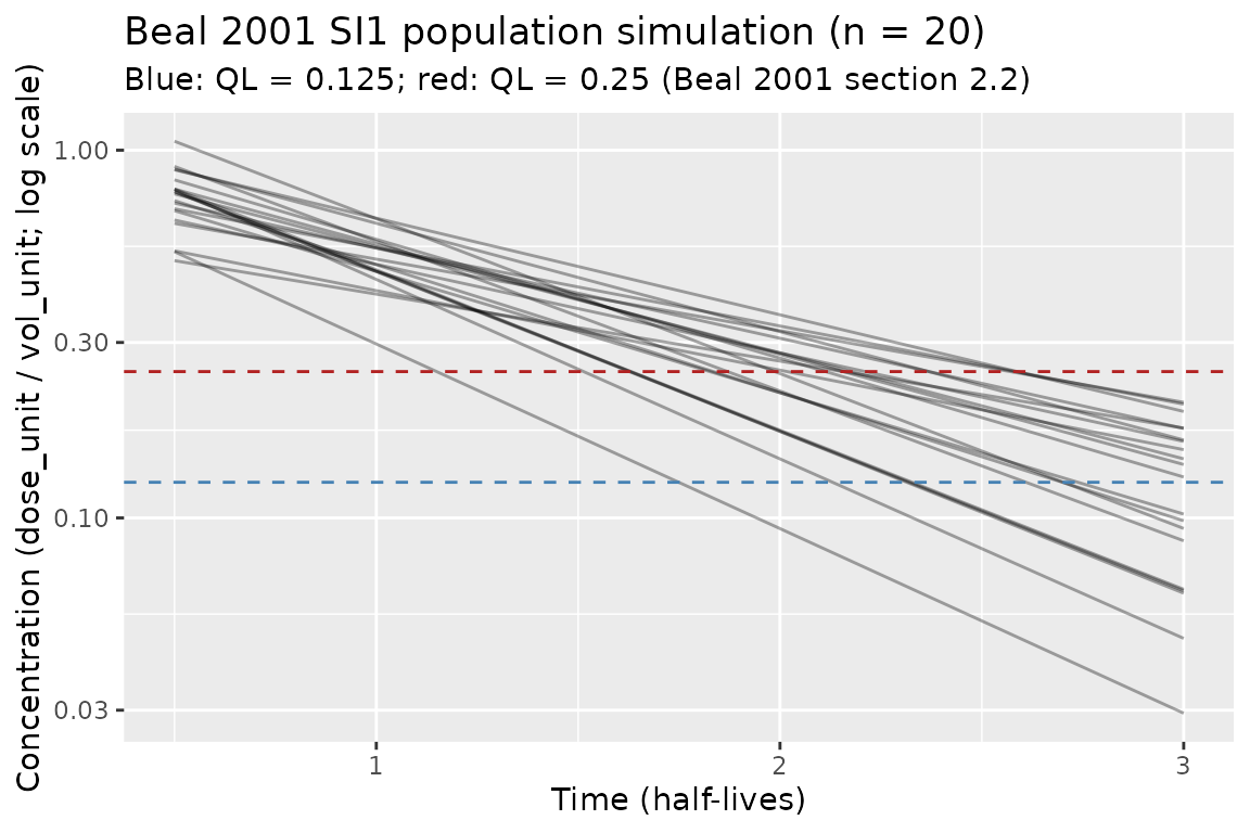
The paper considers two quantification limits:
QL = 0.125 and QL = 0.25 (section 2.2, page
486). For the typical individual QL = 0.125 coincides with
C(t = 3), so about half of the observations at
t = 3 are expected to fall BQL after adding residual error.
Under QL = 0.25 the situation is much harsher:
QL = C(t = 2), so t = 2 is the boundary at
which roughly half of observations fall BQL, and by t = 2.5
almost all observations are BQL.
bql_summary <- sim_df |>
  dplyr::mutate(
    bql_0.125 = Cc < 0.125,
    bql_0.25  = Cc < 0.25
  ) |>
  dplyr::group_by(time) |>
  dplyr::summarise(
    n            = dplyr::n(),
    frac_lt_0.125 = mean(bql_0.125),
    frac_lt_0.25  = mean(bql_0.25),
    .groups       = "drop"
  )

knitr::kable(
  bql_summary,
  digits  = 3,
  caption = paste(
    "Observed fraction of simulated concentrations falling below QL = 0.125",
    "and QL = 0.25, by observation time. Compare with section 2.2 of Beal 2001",
    "(BQL frequencies for the typical individual)."
  )
)| time | n | frac_lt_0.125 | frac_lt_0.25 |
|---|---|---|---|
| 0.5 | 20 | 0.00 | 0.00 |
| 1.0 | 20 | 0.00 | 0.00 |
| 1.5 | 20 | 0.00 | 0.05 |
| 2.0 | 20 | 0.05 | 0.45 |
| 2.5 | 20 | 0.25 | 0.85 |
| 3.0 | 20 | 0.45 | 1.00 |
Visual: simulated profiles under SI1
ggplot(sim_df, aes(x = time, y = Cc, group = id)) +
  geom_line(alpha = 0.35) +
  geom_hline(yintercept = 0.125, linetype = "dashed", colour = "steelblue") +
  geom_hline(yintercept = 0.25,  linetype = "dashed", colour = "firebrick") +
  scale_y_log10() +
  labs(
    x        = "Time (half-lives)",
    y        = "Concentration (dose_unit / vol_unit; log scale)",
    title    = "Beal 2001 SI1 population simulation (n = 20)",
    subtitle = "Blue: QL = 0.125; red: QL = 0.25 (Beal 2001 section 2.2)"
  )
PKNCA sanity check
PKNCA on the typical-individual profile (with a defensively added
t = 0 anchor row at Cc = 1, the paper’s
initial condition) recovers AUC0-inf close to the analytic
1/CL = 1.4429 and terminal half-life close to
1 half-life, confirming that the packaged model behaves
dimensionally as the paper specifies. PKNCA computes half-life from a
log-linear terminal-phase fit; with only six observations the estimate
is expected to be close to but not exactly equal to 1.
sim_typ_nca <- sim_typ |>
  dplyr::select(time, Cc) |>
  dplyr::mutate(id = 1L, treatment = "typical")

sim_typ_nca <- dplyr::bind_rows(
  sim_typ_nca,
  tibble::tibble(id = 1L, treatment = "typical", time = 0, Cc = 1)
) |>
  dplyr::distinct(id, treatment, time, .keep_all = TRUE) |>
  dplyr::arrange(id, treatment, time)

conc_obj <- PKNCA::PKNCAconc(sim_typ_nca, Cc ~ time | treatment + id)

dose_df <- data.frame(
  id        = 1L,
  time      = 0,
  amt       = 1,
  treatment = "typical"
)
dose_obj <- PKNCA::PKNCAdose(dose_df, amt ~ time | treatment + id)

intervals <- data.frame(
  start      = 0,
  end        = Inf,
  cmax       = TRUE,
  tmax       = TRUE,
  aucinf.obs = TRUE,
  half.life  = TRUE
)

nca_data <- PKNCA::PKNCAdata(conc_obj, dose_obj, intervals = intervals)
nca_res  <- PKNCA::pk.nca(nca_data)

as.data.frame(nca_res) |>
  dplyr::select(treatment, PPTESTCD, PPORRES) |>
  knitr::kable(
    digits  = 4,
    caption = paste(
      "PKNCA on the typical individual. Expect AUC0-inf ~ 1/0.693 = 1.4429",
      "and half.life ~ 1 (log(2)/0.693 = 1 by construction). Cmax is dose/Vd = 1",
      "with tmax = 0 for an IV bolus."
    )
)| treatment | PPTESTCD | PPORRES |
|---|---|---|
| typical | cmax | 1.0000 |
| typical | tmax | 0.0000 |
| typical | tlast | 3.0000 |
| typical | clast.obs | 0.1251 |
| typical | lambda.z | 0.6930 |
| typical | r.squared | 1.0000 |
| typical | adj.r.squared | 1.0000 |
| typical | lambda.z.time.first | 0.5000 |
| typical | lambda.z.time.last | 3.0000 |
| typical | lambda.z.n.points | 6.0000 |
| typical | clast.pred | 0.1251 |
| typical | half.life | 1.0002 |
| typical | span.ratio | 2.4995 |
| typical | aucinf.obs | 1.4430 |
Assumptions and deviations
-
Scope. This is a methodology-reference model, not a
drug-specific popPK model. The typical values
CL = 0.693andVd = 1are scale-fixed teaching constants (Beal 2001 section 2.2); they are not estimates of any real molecule and should not be reinterpreted as one. This deviation from the usualspecificDrugs/convention was approved by the maintainers. -
Which omega set. The paper studies two geometric-SD
sets on CL:
omega_CL = 0.2(first set) andomega_CL = 0.4(second set); Vd always usesomega_Vd = 0.2. The encoded model uses the first set because it is introduced first and is used as the reference throughout the paper’s results tables. A downstream user can replace the fixed IIV block with~ fixed(0.16)(i.e.0.4^2) to reproduce the second set. -
Which residual model. The paper studies two
data-analytic variance models (DA1 homogeneous, DA2 constant-CV) and
four simulation variance structures (SI1-SI4). The encoded model uses
the SI1 generative variance (
g(t) = 0.02, homogeneous) as an additive residual, which matches the DA1 analytic pair. Users who want to reproduce SI2/SI3/SI4 or DA2 should modify the residual block accordingly (see section 2.2 of the paper for the SI2-SI4 variance specifications). - No BQL censoring in the packaged model. The BQL handling is what the paper studies; the packaged model is the underlying generative process. Downstream users experimenting with M1-M7 apply their choice of censoring rule on top of the simulated concentrations produced here.
-
PKNCA time-zero anchor. IV-bolus profiles
technically start at
t = 0+withCc = dose/Vd. The PKNCA chunk adds an explicitt = 0, Cc = 1row so the AUC computation is anchored at the correct initial condition; without it PKNCA emits a “Requesting an AUC range starting (0) before the first measurement” warning.