Immune-related adverse events of checkpoint inhibitors in NSCLC (Zhang 2022)
Source:vignettes/articles/Zhang_2022_ici_irae_nsclc_mbma.Rmd
Zhang_2022_ici_irae_nsclc_mbma.RmdModel and source
Zhang et al. pooled trial-level immune-related adverse event (irAE) rates from 129 cohorts of patients with non-small cell lung cancer (NSCLC) treated with immune checkpoint inhibitors (ICIs): the anti-PD-1 antibodies nivolumab and pembrolizumab, the anti-PD-L1 antibodies atezolizumab, durvalumab and avelumab, and the anti-CTLA-4 antibodies ipilimumab and tremelimumab. Each cohort’s regimen was converted to a steady-state average plasma concentration with a published population PK model and divided by the antibody’s in vitro IC50 to give a normalized exposure. Logit-transformed irAE rates were then regressed on normalized exposure, the drug class and trial-level covariates.
- Article: https://doi.org/10.1002/psp4.12834 (PMC9381889), CPT Pharmacometrics Syst Pharmacol. 2022;11(8):1135-1146.
- Supporting Information: Supplementary Tables S1-S7 (Table S3 holds the PK parameters and IC50 values) and the authors’ cohort-level analysis dataset.
The paper’s final models are two study-level logit meta-regressions with no time axis, one per endpoint:
| Model | Endpoint | Source |
|---|---|---|
Zhang_2022_ici_irae_mbma |
any-grade irAE | Equation 4, Table 3 (126 cohorts) |
Zhang_2022_ici_irae_grade3_mbma |
grade >= 3 irAE | Equation 5, Table 3 (120 cohorts) |
mod_names <- c(
  any = "Zhang_2022_ici_irae_mbma",
  g3 = "Zhang_2022_ici_irae_grade3_mbma"
)
mods <- lapply(mod_names, function(n) rxode2::rxode(readModelDb(n)))
coefs <- lapply(mods, function(m) stats::setNames(m$iniDf$est, m$iniDf$name))
Structure
Anti-PD-(L)1 exposure was not associated with either endpoint, so the anti-PD-1 and anti-PD-L1 classes enter as indicators. Only anti-CTLA-4 exposure enters continuously:
Here
is the normalized anti-CTLA-4 exposure (CAV / IC50_CTLA4).
(TRT_ANTIPD1) and
(TRT_ANTIPDL1) are 1 when the regimen contains an antibody
of that class.
is 1 when it contains an anti-CTLA-4 antibody, which the models derive
as CAV > 0. line2+ is formed as
1 - LINE_1L. The paper’s single chemo/target indicator is
formed as max(CONMED_CHEMO, CONMED_NONCHEMO_OTHER). The
intercept is the rate for first-line anti-PD-1 monotherapy.
Population
The analysis included 81 studies with 19,322 patients published up to April 30, 2021: 53 randomized controlled trials, 18 dose-escalation trials, 21 single-arm trials, 20 nonrandomized trials and 17 real-world studies (Results, “Literature data”). By drug class, there were 73 anti-PD-1, 33-36 anti-PD-L1, 5 anti-CTLA-4, 10 anti-CTLA-4 + anti-PD-1 and 5 anti-CTLA-4 + anti-PD-L1 cohorts (Table 1). Supplementary Table S6 summarizes the cohort characteristics:
- median cohort age 64.3 years (range 50-72);
- median 61.8% male;
- median 56.3% PD-L1 positive;
- median 85.0% current or former smokers;
- median 81.8% stage IV;
- median 25.8% squamous histology.
51 cohorts were first-line and 62 second-line or later; the rest were imputed or rounded. 71 were ICI monotherapy, 34 added chemotherapy and 12 added targeted therapy. Age, sex, PD-L1 status, smoking, stage, histology and the individual drug within a target class were screened and not retained.
The same information is available programmatically via each model’s
population metadata,
e.g. rxode2::rxode(readModelDb("Zhang_2022_ici_irae_mbma"))$population.
Source trace
| Equation / parameter | Value | Source location |
|---|---|---|
| Any-grade final model | n/a | Methods, “Statistical analysis”, Equation 4 |
| Grade >= 3 final model | n/a | Methods, “Statistical analysis”, Equation 5 |
| Indicator definitions (Factor_PD-1, Factor_PD-L1, Factor_CTLA-4) | n/a | Methods, text after Equation 3 |
cnorm_ctla4 <- CAV / IC50_CTLA4 |
n/a | Methods, “ICI exposure normalization”; Table S3 |
any logit_ref
() |
-1.2696 | Table 3, any grade |
any e_antipdl1_logit
() |
-0.3484 | Table 3, any grade |
any e_cnorm_ctla4_logit
() |
0.0013 | Table 3, any grade |
any e_line2_logit
() |
-0.4757 | Table 3, any grade |
any e_chemo_target_logit
() |
0.9093 | Table 3, any grade |
grade >= 3 logit_ref
() |
-3.1445 | Table 3, grade >= 3 |
grade >= 3 e_antipdl1_logit
() |
-0.6271 | Table 3, grade >= 3 |
grade >= 3 e_cnorm_ctla4_logit
() |
0.0014 | Table 3, grade >= 3 |
grade >= 3 e_cnorm_ctla4_antipd1_logit
() |
0.0176 | Table 3, grade >= 3 |
grade >= 3 e_antipdl1_antictla4_logit
() |
1.3525 | Table 3, grade >= 3 |
grade >= 3 e_line2_logit
() |
-0.6285 | Table 3, grade >= 3 |
grade >= 3 e_chemo_target_logit
() |
0.8790 | Table 3, grade >= 3 |
addSd_prob_* |
0.001 (fixed) | not from source; see Assumptions |
| Ipilimumab / tremelimumab PK parameters and IC50 | see table below | Supplementary Table S3 |
| Normalized exposure per anti-CTLA-4 regimen | see table below | Supplementary dataset, column CCTLA4 |
Exposure input
The models do not take a dose. The input is the cohort’s average
anti-CTLA-4 concentration CAV and the antibody’s
IC50_CTLA4, in the same unit. Only their ratio enters.
Table S3 gives the two-compartment PK parameters and IC50 values the
authors used. The paper does not give the body weight for mg/kg doses or
the averaging window. The authors’ supplementary dataset, however, lists
the normalized exposure of every cohort. Those are the values the
coefficients were fitted on, so they are the values to supply.
pk_par <- tibble::tribble(
  ~drug,          ~cl,   ~vc,  ~q,    ~vp,  ~ic50,
  "ipilimumab",   0.360, 4.15, 0.986, 3.11, 200,
  "tremelimumab", 0.262, 3.72, 0.413, 3.31, 95.15
)
pk_par |>
  dplyr::rename(
    Drug = drug, "CL (L/day)" = cl, "Vc (L)" = vc, "Q (L/day)" = q,
    "Vp (L)" = vp, "IC50 (ng/mL)" = ic50
  ) |>
knitr::kable(caption = "Supplementary Table S3 of Zhang 2022 (anti-CTLA-4 rows).")| Drug | CL (L/day) | Vc (L) | Q (L/day) | Vp (L) | IC50 (ng/mL) |
|---|---|---|---|---|---|
| ipilimumab | 0.360 | 4.15 | 0.986 | 3.11 | 200.00 |
| tremelimumab | 0.262 | 3.72 | 0.413 | 3.31 | 95.15 |
regimens <- tibble::tribble(
  ~regimen,                    ~drug,          ~mgkg, ~tau, ~cnorm_dataset,
  "ipilimumab 1 mg/kg Q12W",   "ipilimumab",   1,     84,   8,
  "ipilimumab 1 mg/kg Q6W",    "ipilimumab",   1,     42,   17.5,
  "ipilimumab 1 mg/kg Q3W",    "ipilimumab",   1,     21,   36,
  "ipilimumab 3 mg/kg Q3W",    "ipilimumab",   3,     21,   109,
  "ipilimumab 10 mg/kg Q3W",   "ipilimumab",   10,    21,   375,
  "tremelimumab 1 mg/kg Q4W",  "tremelimumab", 1,     28,   115.61,
  "tremelimumab 3 mg/kg Q4W",  "tremelimumab", 3,     28,   346.83,
  "tremelimumab 10 mg/kg Q4W", "tremelimumab", 10,    28,   1156.1
) |>
  dplyr::left_join(pk_par, by = "drug") |>
  dplyr::mutate(id = dplyr::row_number())
To show how these values relate to Table S3, each regimen is
simulated at 70 kg with the Table S3 parameters. PKNCA computes the
average concentration over the interval between the 3rd and 4th doses.
The closed-form steady-state value Dose / (CL * tau) is
shown alongside.
pk_mod <- rxode2::rxode2({
  d / dt(central) <- -cl / vc * central - q / vc * central + q / vp * peripheral1
  d / dt(peripheral1) <- q / vc * central - q / vp * peripheral1
  Cc <- 1000 * central / vc # ng/mL from mg and L
})
wt <- 70 # kg; see Assumptions

sim_one <- function(r) {
  obs_times <- sort(unique(c(seq(0, 4 * r$tau, length.out = 801), 2 * r$tau, 3 * r$tau)))
  ev <- rxode2::et(amt = r$mgkg * wt, ii = r$tau, addl = 3, cmt = "central") |>
    rxode2::et(obs_times, cmt = "central")
  s <- rxode2::rxSolve(
    pk_mod,
    params = c(cl = r$cl, vc = r$vc, q = r$q, vp = r$vp),
    events = ev, returnType = "data.frame"
  )
  data.frame(id = r$id, regimen = r$regimen, time = s$time, Cc = s$Cc)
}
conc <- dplyr::bind_rows(lapply(split(regimens, regimens$id), sim_one))
dose_df <- dplyr::bind_rows(lapply(split(regimens, regimens$id), function(r) {
  data.frame(id = r$id, regimen = r$regimen, time = r$tau * 0:3, amt = r$mgkg * wt)
}))

conc_obj <- PKNCA::PKNCAconc(
  dplyr::filter(conc, !is.na(Cc)), Cc ~ time | regimen + id,
  concu = "ng/mL", timeu = "day"
)
dose_obj <- PKNCA::PKNCAdose(dose_df, amt ~ time | regimen + id, doseu = "mg")
intervals <- regimens |>
  dplyr::transmute(regimen, id, start = 2 * tau, end = 3 * tau, cav = TRUE)
nca <- PKNCA::pk.nca(PKNCA::PKNCAdata(conc_obj, dose_obj, intervals = intervals))

cav <- as.data.frame(nca$result) |>
  dplyr::filter(PPTESTCD == "cav") |>
  dplyr::select(id, cav_d34 = PPORRES)

exposure <- regimens |>
  dplyr::left_join(cav, by = "id") |>
  dplyr::mutate(
    cav_ss = 1000 * mgkg * wt / (cl * tau),
    cnorm_d34 = cav_d34 / ic50,
    cnorm_ss = cav_ss / ic50,
    ratio = cnorm_dataset / cnorm_ss,
    CAV = cnorm_dataset * ic50
  )

exposure |>
  dplyr::select(regimen, cnorm_d34, cnorm_ss, cnorm_dataset, ratio, CAV) |>
  dplyr::mutate(dplyr::across(where(is.numeric), ~ signif(.x, 3))) |>
  dplyr::rename(
    Regimen = regimen,
    "Cav/IC50, doses 3-4 at 70 kg" = cnorm_d34,
    "Cav/IC50, Dose/(CL tau) at 70 kg" = cnorm_ss,
    "Cav/IC50, authors' dataset" = cnorm_dataset,
    "Dataset / steady state" = ratio,
    "CAV to supply (ng/mL)" = CAV
  ) |>
knitr::kable(caption = "Normalized anti-CTLA-4 exposure by regimen.")| Regimen | Cav/IC50, doses 3-4 at 70 kg | Cav/IC50, Dose/(CL tau) at 70 kg | Cav/IC50, authors’ dataset | Dataset / steady state | CAV to supply (ng/mL) |
|---|---|---|---|---|---|
| ipilimumab 1 mg/kg Q12W | 11.8 | 11.6 | 8.0 | 0.691 | 1600 |
| ipilimumab 1 mg/kg Q6W | 23.3 | 23.1 | 17.5 | 0.756 | 3500 |
| ipilimumab 1 mg/kg Q3W | 44.2 | 46.3 | 36.0 | 0.778 | 7200 |
| ipilimumab 3 mg/kg Q3W | 133.0 | 139.0 | 109.0 | 0.785 | 21800 |
| ipilimumab 10 mg/kg Q3W | 442.0 | 463.0 | 375.0 | 0.810 | 75000 |
| tremelimumab 1 mg/kg Q4W | 95.1 | 100.0 | 116.0 | 1.150 | 11000 |
| tremelimumab 3 mg/kg Q4W | 285.0 | 301.0 | 347.0 | 1.150 | 33000 |
| tremelimumab 10 mg/kg Q4W | 951.0 | 1000.0 | 1160.0 | 1.150 | 110000 |
ipi <- dplyr::filter(exposure, drug == "ipilimumab")
tre <- dplyr::filter(exposure, drug == "tremelimumab")
stopifnot(
  # The 3rd-4th interval average does not exceed steady state beyond
  # trapezoidal error.
  all(exposure$cnorm_d34 < exposure$cnorm_ss * 1.02),
  # The authors' ipilimumab values sit 0.65-0.85 times the 70 kg steady state,
  # and their tremelimumab values are dose-proportional at about 1.15 times it.
  all(ipi$ratio > 0.65 & ipi$ratio < 0.85),
  all(abs(tre$ratio - 1.153) < 0.005)
)
Neither averaging convention at 70 kg reproduces the authors’ values. The ipilimumab values are 0.69-0.81 times steady state and do not scale exactly with dose / interval. The tremelimumab values are exactly dose-proportional but 1.15 times steady state. The maintainers could not find a single body weight or averaging window that gives both. Use the dataset values (the last column) for these regimens. For other regimens, the closed-form steady state is the nearest documented approximation, and it puts ipilimumab exposure 25-45% higher than the fitted axis.
Replicating Figure 4
Figure 4 of the paper prints the model-predicted any-grade and grade >= 3 irAE rates for the following scenarios:
- first- vs second-line anti-PD-1 (a) and anti-PD-L1 (b) therapy, alone or with chemotherapy / targeted therapy;
- first-line ipilimumab (c), at 1 mg/kg Q6W or Q3W with an anti-PD-1 antibody, or at 3 or 10 mg/kg Q3W with chemotherapy / targeted therapy.
All 24 printed values are reproduced from the Table 3 coefficients.
ipi_cnorm <- stats::setNames(ipi$cnorm_dataset, ipi$regimen)
scen <- tibble::tribble(
  ~panel, ~scenario, ~TRT_ANTIPD1, ~TRT_ANTIPDL1, ~LINE_1L, ~CONMED_CHEMO, ~cnorm,
  "(a) PD-1", "1st line monotherapy", 1, 0, 1, 0, 0,
  "(a) PD-1", "2nd line monotherapy", 1, 0, 0, 0, 0,
  "(a) PD-1", "1st line with chemo/target", 1, 0, 1, 1, 0,
  "(a) PD-1", "2nd line with chemo/target", 1, 0, 0, 1, 0,
  "(b) PD-L1", "1st line monotherapy", 0, 1, 1, 0, 0,
  "(b) PD-L1", "2nd line monotherapy", 0, 1, 0, 0, 0,
  "(b) PD-L1", "1st line with chemo/target", 0, 1, 1, 1, 0,
  "(b) PD-L1", "2nd line with chemo/target", 0, 1, 0, 1, 0,
  "(c) CTLA-4", "1 mg/kg Q6W with PD-1 inhibitor", 1, 0, 1, 0,
  ipi_cnorm[["ipilimumab 1 mg/kg Q6W"]],
  "(c) CTLA-4", "1 mg/kg Q3W with PD-1 inhibitor", 1, 0, 1, 0,
  ipi_cnorm[["ipilimumab 1 mg/kg Q3W"]],
  "(c) CTLA-4", "3 mg/kg Q3W with chemo/target", 0, 0, 1, 1,
  ipi_cnorm[["ipilimumab 3 mg/kg Q3W"]],
  "(c) CTLA-4", "10 mg/kg Q3W with chemo/target", 0, 0, 1, 1,
  ipi_cnorm[["ipilimumab 10 mg/kg Q3W"]]
) |>
  dplyr::mutate(
    id = dplyr::row_number(), time = 0, IC50_CTLA4 = 200,
    CAV = cnorm * IC50_CTLA4, CONMED_NONCHEMO_OTHER = 0,
    # Figure 4 of Zhang 2022, printed labels
    any_printed = c(21.9, 14.9, 41.1, 30.2, 16.5, 11.0, 33.0, 23.4, 22.3, 22.7, 44.6, 53.2),
    g3_printed = c(4.13, 2.25, 9.40, 5.25, 2.25, 1.21, 5.25, 2.87, 5.67, 7.87, 10.8, 14.9)
  )

cov_cols <- c(
  "id", "time", "TRT_ANTIPD1", "TRT_ANTIPDL1", "LINE_1L", "CONMED_CHEMO",
  "CONMED_NONCHEMO_OTHER", "CAV", "IC50_CTLA4"
)
solve_prob <- function(mod, data) {
  d <- data[, cov_cols]
  s <- rxode2::rxSolve(mod, d, returnType = "data.frame")
  s[, grep("^prob_", names(s))[1]]
}
scen$any_model <- 100 * solve_prob(mods$any, scen)
#> Warning: multi-subject simulation without without 'omega'
scen$g3_model <- 100 * solve_prob(mods$g3, scen)
#> Warning: multi-subject simulation without without 'omega'

scen |>
  dplyr::mutate(dplyr::across(c(any_model, g3_model), ~ round(.x, 2))) |>
  dplyr::select(panel, scenario, any_model, any_printed, g3_model, g3_printed) |>
  dplyr::rename(
    Panel = panel, Scenario = scenario,
    "Any grade, model (%)" = any_model, "Any grade, Figure 4 (%)" = any_printed,
    "Grade >= 3, model (%)" = g3_model, "Grade >= 3, Figure 4 (%)" = g3_printed
  ) |>
knitr::kable(caption = "Model predictions vs. the values printed in Figure 4.")| Panel | Scenario | Any grade, model (%) | Any grade, Figure 4 (%) | Grade >= 3, model (%) | Grade >= 3, Figure 4 (%) |
|---|---|---|---|---|---|
| (a) PD-1 | 1st line monotherapy | 21.93 | 21.9 | 4.13 | 4.13 |
| (a) PD-1 | 2nd line monotherapy | 14.86 | 14.9 | 2.25 | 2.25 |
| (a) PD-1 | 1st line with chemo/target | 41.09 | 41.1 | 9.40 | 9.40 |
| (a) PD-1 | 2nd line with chemo/target | 30.24 | 30.2 | 5.25 | 5.25 |
| (b) PD-L1 | 1st line monotherapy | 16.55 | 16.5 | 2.25 | 2.25 |
| (b) PD-L1 | 2nd line monotherapy | 10.97 | 11.0 | 1.21 | 1.21 |
| (b) PD-L1 | 1st line with chemo/target | 32.99 | 33.0 | 5.25 | 5.25 |
| (b) PD-L1 | 2nd line with chemo/target | 23.43 | 23.4 | 2.87 | 2.87 |
| (c) CTLA-4 | 1 mg/kg Q6W with PD-1 inhibitor | 22.32 | 22.3 | 5.67 | 5.67 |
| (c) CTLA-4 | 1 mg/kg Q3W with PD-1 inhibitor | 22.74 | 22.7 | 7.87 | 7.87 |
| (c) CTLA-4 | 3 mg/kg Q3W with chemo/target | 44.56 | 44.6 | 10.78 | 10.80 |
| (c) CTLA-4 | 10 mg/kg Q3W with chemo/target | 53.18 | 53.2 | 14.92 | 14.90 |
# Deterministic: no cohort, no random draws. The printed labels carry 3
# significant figures, so the bound is the resolution of the printed values.
stopifnot(
  all(abs(scen$any_model - scen$any_printed) < 0.06),
  all(abs(scen$g3_model - scen$g3_printed) < 0.06)
)
scen |>
  dplyr::select(panel, scenario, any_model, g3_model) |>
  tidyr::pivot_longer(c(any_model, g3_model), names_to = "endpoint", values_to = "p") |>
  dplyr::mutate(
    endpoint = ifelse(endpoint == "any_model", "Any grade", "Grade >= 3"),
    scenario = factor(scenario, levels = unique(scen$scenario))
  ) |>
  ggplot(aes(scenario, p, colour = endpoint)) +
  geom_point(size = 2.5) +
  geom_text(aes(label = signif(p, 3)), hjust = -0.3, size = 3, show.legend = FALSE) +
  facet_wrap(~panel, ncol = 2, scales = "free") +
  scale_colour_manual(values = c("Any grade" = "blue", "Grade >= 3" = "red")) +
  labs(x = NULL, y = "Model predicted irAE rate (%)", colour = NULL) +
  theme_bw() +
  theme(axis.text.x = element_text(angle = 30, hjust = 1), legend.position = "bottom")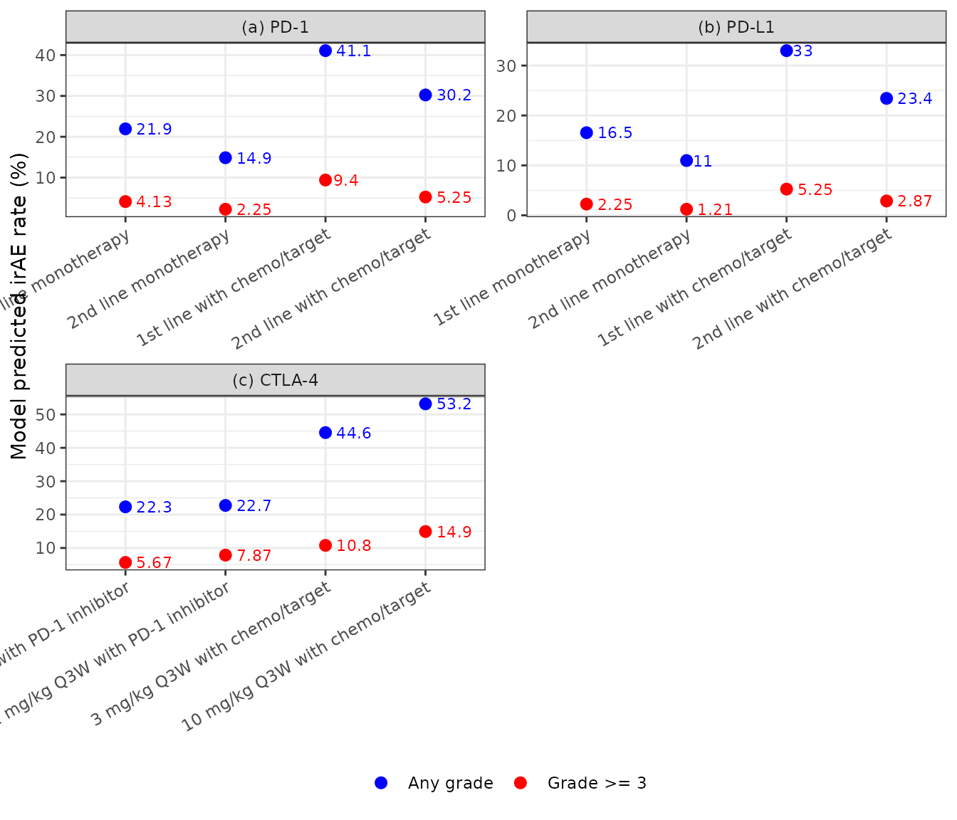
Replicates Figure 4 of Zhang 2022 (point predictions; the paper’s 95% confidence intervals need the coefficient covariance, which is not published).
Exposure dependence
Figure 2e,f plots the irAE rates against normalized anti-CTLA-4 exposure. The curves below show the typical first-line predictions without chemotherapy or targeted therapy for anti-CTLA-4 monotherapy and its combinations. Panel (a) is any grade; panel (b) is grade >= 3, where the anti-PD-1 combination steepens the slope and the anti-PD-L1 combination raises the baseline.
grid <- tidyr::expand_grid(
  cnorm = seq(0, 1200, by = 10),
  combo = c("CTLA-4 monotherapy", "CTLA-4 + PD-1", "CTLA-4 + PD-L1")
) |>
  dplyr::filter(combo != "CTLA-4 + PD-1" | cnorm <= 120) |>
  dplyr::mutate(
    id = dplyr::row_number(), time = 0, IC50_CTLA4 = 1, CAV = cnorm,
    TRT_ANTIPD1 = as.numeric(combo == "CTLA-4 + PD-1"),
    TRT_ANTIPDL1 = as.numeric(combo == "CTLA-4 + PD-L1"),
    LINE_1L = 1, CONMED_CHEMO = 0, CONMED_NONCHEMO_OTHER = 0
  )
grid$any <- 100 * solve_prob(mods$any, grid)
#> Warning: multi-subject simulation without without 'omega'
grid$g3 <- 100 * solve_prob(mods$g3, grid)
#> Warning: multi-subject simulation without without 'omega'

grid |>
  tidyr::pivot_longer(c(any, g3), names_to = "endpoint", values_to = "p") |>
  dplyr::mutate(endpoint = ifelse(endpoint == "any", "(a) any grade", "(b) grade >= 3")) |>
  ggplot(aes(cnorm, p, colour = combo)) +
  geom_line(linewidth = 1) +
  facet_wrap(~endpoint, scales = "free_y") +
  labs(
    x = "CTLA-4 normalized exposure (Cav / IC50)", y = "irAE rate (%)",
    colour = NULL
  ) +
  theme_bw() +
  theme(legend.position = "bottom")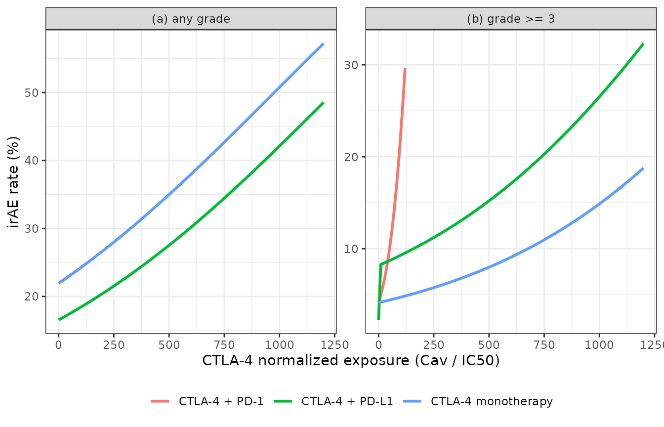
The anti-CTLA-4 + anti-PD-1 curves are drawn only up to a normalized exposure of 120, just above the highest combination cohort (109). The anti-CTLA-4 + anti-PD-L1 curve in panel (a) coincides with the anti-PD-L1 shift alone, because the any-grade model has no combination term.
# Table 3 odds ratios are exp(beta) of the printed coefficients.
or_tab <- tibble::tribble(
  ~model, ~parameter,                    ~or_printed,
  "any",  "e_antipdl1_logit",            0.7058,
  "any",  "e_cnorm_ctla4_logit",         1.0013,
  "any",  "e_line2_logit",               0.6215,
  "any",  "e_chemo_target_logit",        2.4826,
  "g3",   "e_antipdl1_logit",            0.5341,
  "g3",   "e_cnorm_ctla4_logit",         1.0014,
  "g3",   "e_cnorm_ctla4_antipd1_logit", 1.0178,
  "g3",   "e_antipdl1_antictla4_logit",  3.8671,
  "g3",   "e_line2_logit",               0.5334,
  "g3",   "e_chemo_target_logit",        2.4085
)
or_tab$or_model <- mapply(function(m, p) exp(coefs[[m]][[p]]), or_tab$model, or_tab$parameter)
or_tab |>
  dplyr::mutate(or_model = round(or_model, 4)) |>
  dplyr::rename(
    Model = model, Parameter = parameter,
    "OR, Table 3" = or_printed, "OR, exp(coefficient)" = or_model
  ) |>
knitr::kable(caption = "Odds ratios in Table 3 vs. exp() of the encoded coefficients.")| Model | Parameter | OR, Table 3 | OR, exp(coefficient) |
|---|---|---|---|
| any | e_antipdl1_logit | 0.7058 | 0.7058 |
| any | e_cnorm_ctla4_logit | 1.0013 | 1.0013 |
| any | e_line2_logit | 0.6215 | 0.6214 |
| any | e_chemo_target_logit | 2.4826 | 2.4826 |
| g3 | e_antipdl1_logit | 0.5341 | 0.5341 |
| g3 | e_cnorm_ctla4_logit | 1.0014 | 1.0014 |
| g3 | e_cnorm_ctla4_antipd1_logit | 1.0178 | 1.0178 |
| g3 | e_antipdl1_antictla4_logit | 3.8671 | 3.8671 |
| g3 | e_line2_logit | 0.5334 | 0.5334 |
| g3 | e_chemo_target_logit | 2.4085 | 2.4085 |
Assumptions and deviations
-
Study-level model. Both models predict the expected
irAE proportion of a trial cohort; they are not individual-patient risk
models. There is no time axis and no dose event: exposure enters as the
covariate columns
CAVandIC50_CTLA4. -
No residual or between-cohort variance. The paper
fits generalized linear mixed meta-regressions with a random cohort
intercept and does not report the between-cohort variance. Each model
carries a placeholder additive residual
addSd_prob_* = fixed(0.001)so rxode2 has an error model; it is not a published quantity. Read theprob_*column for typical-value predictions. The maintainers refitted Equations 2-5 to the authors’ supplementary dataset as a binomial mixed model with a random cohort intercept (lme4::glmer, 7-point adaptive quadrature). The fixed effects reproduced Tables 2 and 3 to all four printed decimals. The between-cohort SD of the logit intercept from that refit was 0.69 (any grade) and 0.46 (grade >= 3). These values are not encoded in the models because the paper does not report them. Because of the random intercept,expit()of the linear predictor is the median-cohort rate, which is how Figure 4 reports it, rather than the mean across cohorts. -
Exposure input. Supply
CAVandIC50_CTLA4in the same unit. The models document ng/mL, as Table S3 prints the IC50 values. For the anti-CTLA-4 regimens in the analysis, use the authors’ normalized exposures (see “Exposure input”). The 70 kg simulations above only illustrate how those values relate to Table S3. -
Anti-CTLA-4 indicator. The paper’s Factor_CTLA-4
enters only through its product with Factor_PD-L1, i.e. it marks the
anti-CTLA-4 + anti-PD-L1 combination. The grade >= 3 model derives it
as
CAV > 0rather than taking a separate column, so a regimen with an anti-CTLA-4 antibody must have a positiveCAV. -
Chemotherapy or targeted therapy. The paper fits
one coefficient for combination with chemotherapy or targeted therapy.
It is encoded through the two indicators
CONMED_CHEMOandCONMED_NONCHEMO_OTHER, combined withmax(). The targeted agents are not named individually in Supplementary Table S4. -
Line of therapy. The source covariate line2+ is
encoded through the canonical
LINE_1Las1 - LINE_1L. Cohorts that mixed lines were rounded to 0 or 1 by the majority line, and missing values were imputed; the models are defined only forLINE_1Lequal to 0 or 1.
Errata
- Figure 4c vs. Methods. Methods (“Model simulation”) lists the simulated ipilimumab regimens with chemotherapy / targeted therapy as “1 or 10 mg/kg Q3W”; Figure 4c labels them 3 mg/kg and 10 mg/kg Q3W. The printed Figure 4c values (44.6% and 10.8%) are reproduced only with the 3 mg/kg Q3W normalized exposure (109), so the figure label is correct and the Methods text is not.
- Table 3, any-grade standard error. Table 3 prints SE 1.2124 with 95% CI [0.6061, 1.1893] and p < 0.0001 for the chemo/target coefficient 0.9093. An SE of 1.2124 is inconsistent with that CI and p-value. The maintainers’ refit gives SE 0.1547 and CI [0.606, 1.213]; the printed upper bound repeats the grade >= 3 row. The point estimate is unaffected.
- Table 2, any-grade CI. The base-model any-grade (-0.3862, SE 0.1837) carries the CI [-1.0287, -0.1825] of the grade >= 3 row below it; -0.3862 +/- 1.96 x 0.1837 gives [-0.746, -0.026]. The base model is not shipped.
- Factor_CTLA-4 definition. Methods says Factor_CTLA-4 “is set to 1 only if a CTLA-4 inhibitor was given with a PD-L1 inhibitor”. The supplementary dataset sets it to 1 for every anti-CTLA-4 regimen. The two readings give identical predictions because the factor appears only in the product with Factor_PD-L1.
- Checked on 2026-10-05: no erratum or correction for this article was found.