In vitro multilineage hematopoiesis and drug-induced cytopenia (Wilson 2020)
Source:vignettes/articles/Wilson_2020_hematopoiesis_invitro.Rmd
Wilson_2020_hematopoiesis_invitro.RmdModel and source
mod <- readModelDb("Wilson_2020_hematopoiesis_invitro")
ui <- rxode2::rxode2(mod)
drugPar <- ui$meta$drugEffectParameters
names(drugPar)
#>  [1] "abemaciclib"  "dinaciclib"   "docetaxel"    "paclitaxel"   "palbociclib"
#>  [6] "pictilisib"   "ribociclib"   "thalidomide"  "fluorouracil" "A_1331852"
#> [11] "bortezomib" "cytarabine" "lenalidomide" "OTX015"- Citation: Wilson JL, Lu D, Corr N, Fullerton A, Lu J. An in vitro quantitative systems pharmacology approach for deconvolving mechanisms of drug-induced, multilineage cytopenias. PLoS Comput Biol 2020;16(7):e1007620. https://doi.org/10.1371/journal.pcbi.1007620 (open access, PMC7402526).
- Supporting information used here: S1 Text (the SimBiology export of every flux, ODE, rule, event and parameter value), S3 Text (the mapping between the Greek-letter names of the figures and the MATLAB names), S1 Table (the vehicle-normalized day-6 cell counts of the drug-treatment experiment) and S2 Table (the fitted EmaxT and log(EC50) of every compound). The SimBiology project is also deposited at https://github.com/jenwilson521/Multilineage_InvitroHem_Model.
The model describes hematopoiesis in a 6-day culture of human
bone-marrow CD34+ cells (the multilineage toxicity assay, MLTA).
Hematopoietic stem cells (HSC) renew themselves and feed multipotent
progenitors (MPP); MPP branch into granulocyte-macrophage progenitors
(GMP), megakaryocytes (MK), early erythroid cells and lymphoid
progenitors; GMP branch into monocyte and granulocyte progenitors, which
mature into monocytes and granulocytes, and granulocytes feed a
proliferating and a quiescent neutrophil pool. Early erythroid cells
mature into late erythroid cells, and lymphoid progenitors into B cells.
Each division makes two daughters that renew with probability rho or
differentiate with probability 1 - rho (Fig 2B). Only the most mature
cell of each lineage dies, at one shared rate kdeath.
A drug acts on every cell type through one total Emax (EmaxT) and one log(EC50) per cell type. The part of EmaxT up to 1 inhibits the basal proliferation rate; the part above 1 is a first-order kill rate in 1/day:
kpro   = kpro0 * (1 - min(1, EmaxT) * C / (EC50 + C))
kkill  = max(0, EmaxT - 1) * C / (EC50 + C)
The packaged ini() holds the system parameters
calibrated to drug-free kinetics with every drug effect off
(emaxt_* = 0). The fitted drug-effect sets are in
ui$meta$drugEffectParameters, one named vector per
compound, and are passed to rxSolve(params = ).
Population
The system parameters and the 14 initial cell counts were fitted to the mean of six donor samples of CD34+ cells cultured without drug and counted on days 2 to 6 (days 0 and 9 were dropped; see Results, “The model explains cell kinetic data in the absence of drug treatment”). The drug-effect parameters were fitted, one compound at a time, to day-6 counts after exposure to 0.2, 1, 5, 25, 100, 500 and 2500 nM added on day 0, normalized to vehicle-control wells and pooled over 2-7 donor samples (S1 Table). Because the fits are to donor means, the model is deterministic: it carries no between-donor variability and no residual error.
Source trace
| Element | Value(s) | Source |
|---|---|---|
Flux equations (r1 … r32,
kill_*) |
38 fluxes | S1 Text, “Fluxes” |
| ODE stoichiometry (15 cell states + drug) | as printed | S1 Text, “ODEs” |
Anti-proliferation rule
kpro = kpro0 * (1 - min(1, EmaxT) * C/(EC50 + C))
|
12 cell types | S1 Text rules 5-16; Methods Eq 2 |
Cell-kill rule max(0, EmaxT - 1) * C/(EC50 + C)
(1/day) |
13 cell types | S1 Text rules 17-29 and fluxes 25-38; Methods Eq 3 |
Neutrophil quiescent split
QF_Neutrophil * initNeutrophil
|
at t = 0.01 day | S1 Text, “Events” |
totalViableCells, viability,
Neutrophil-lin
|
sums | S1 Text, “Repeated Assignments” |
kpro0_* (12), renew_* (7),
kbranch_* (4), kdeath, kdiff_lym,
qf_neut
|
26 values | S1 Text, “Parameters (Model Scoped)” |
bl_* (14 initial counts) |
cells/mL | S1 Text, “Species - InVitro” (1 mL compartment) |
emaxt_* = 0, lec50_* = 1 (drug-free
defaults) |
26 values | S1 Text, “Parameters (Model Scoped)” |
drugEffectParameters (14 named compounds) |
26 values each | S2 Table, sheet “log_EC50_parameters_from_fittin”; Table 1 (rounded) |
| Parameter-name mapping (rho, kappa, beta, delta) | S3 Text | |
| Day-6 normalized observations used below | 8 compounds | S1 Table |
Drug-free kinetics
Cross-checks against S1 Text
S1 Text lists the initial viability as
0.785724947286575. It is a function of the fitted initial counts alone,
so it checks the 14 bl_* values and the
totalViableCells sum.
evCtl <- et(amt = 0, cmt = "drug", time = 0) |>
  et(seq(0, 6, by = 0.05))
simCtl <- as.data.frame(rxSolve(ui, evCtl))
v0 <- simCtl$viability[simCtl$time == 0]
v0
#> [1] 0.7857249
stopifnot(abs(v0 - 0.785724947286575) < 1e-9)
Replicates Figure 3 of Wilson 2020
cellCols <- c(
  HSC = "hsc", MPP = "mpp", GMP = "gmp", "Gran-lin prog" = "gran_prog",
  "Gran-lin" = "gran", "Monocyte prog" = "mono_prog", "Monocyte-lin" = "mono",
  "Neutrophil-lin" = "neut", "Erythroid-lin I" = "eryth1",
  "Erythroid-lin II" = "eryth2", "MK-lin" = "mk", "Lymphoid prog" = "lym_prog",
  "B-lin" = "bcell", "Total dead cells" = "dead_cells"
)
simCtl |>
  select(time, all_of(cellCols)) |>
  pivot_longer(-time, names_to = "cell", values_to = "count") |>
  mutate(cell = factor(cell, levels = names(cellCols))) |>
  ggplot(aes(time, count)) +
  geom_line(colour = "#C2185B") +
  scale_y_log10(limits = c(1, 1e7)) +
  facet_wrap(~cell, ncol = 4) +
  labs(x = "Time (day)", y = "Cells/mL",
       caption = "Replicates the model lines of Figure 3 of Wilson 2020 (drug-free kinetics).") +
  theme_bw()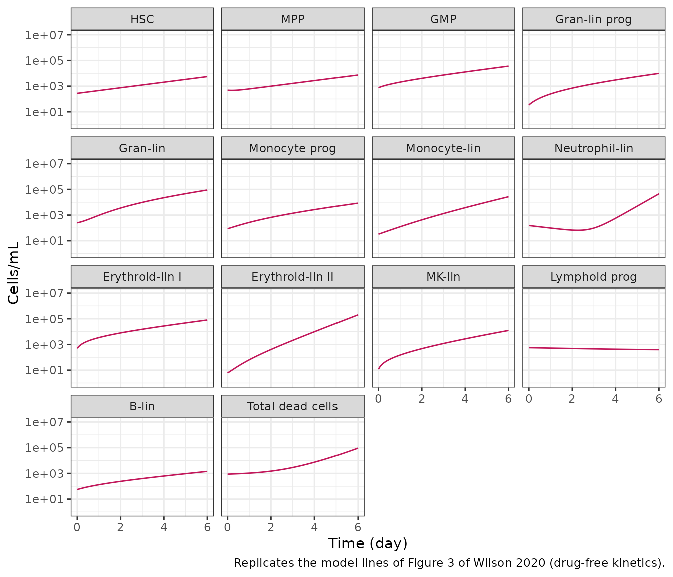
The paper does not print the Figure 3 values. The day-6 end points of its model lines were read by eye from the log-scale panels, to about 0.1 decade, and the packaged model reproduces each one to within 0.3 decade:
fig3Day6 <- c(
  hsc = 3.7, mpp = 3.85, gmp = 4.5, gran_prog = 3.9, gran = 4.9,
  mono_prog = 4.0, mono = 4.5, neut = 4.7, eryth1 = 4.9, eryth2 = 5.2,
  mk = 4.1, lym_prog = 2.7, bcell = 3.2, dead_cells = 4.9
)
simLog6 <- log10(unlist(simCtl[simCtl$time == 6, names(fig3Day6)]))
data.frame(
  cell = names(fig3Day6),
  figure3_log10 = fig3Day6,
  simulated_log10 = round(simLog6, 2)
) |>
  rename("State" = cell, "Figure 3, log10 cells/mL (by eye)" = figure3_log10,
         "Simulated, log10 cells/mL" = simulated_log10) |>
knitr::kable(row.names = FALSE)| State | Figure 3, log10 cells/mL (by eye) | Simulated, log10 cells/mL |
|---|---|---|
| hsc | 3.70 | 3.74 |
| mpp | 3.85 | 3.87 |
| gmp | 4.50 | 4.56 |
| gran_prog | 3.90 | 3.99 |
| gran | 4.90 | 4.95 |
| mono_prog | 4.00 | 3.93 |
| mono | 4.50 | 4.43 |
| neut | 4.70 | 4.66 |
| eryth1 | 4.90 | 4.91 |
| eryth2 | 5.20 | 5.31 |
| mk | 4.10 | 4.09 |
| lym_prog | 2.70 | 2.60 |
| bcell | 3.20 | 3.16 |
| dead_cells | 4.90 | 4.97 |
The shapes also match. Lymphoid progenitors are the only lineage that declines (the Discussion comments on this), and neutrophils dip over the first two days before expanding steeply.
The neutrophil split at t = 0 instead of t = 0.01 day
In SimBiology, the neutrophils start as one proliferating pool of
154.07 cells/mL, and an event at t = 0.01 day moves 99.974% of the
initial count into a quiescent pool. The packaged model applies
the split at t = 0. The exact SimBiology behaviour can be reproduced
with rxode2 replacement events (evid = 5): start with
qf_neut = 0 (everything proliferating) and replace both
pools at t = 0.01 day.
qf <- ui$theta[["qf_neut"]]
n0 <- ui$theta[["bl_neut"]]
evExact <- et(amt = 0, cmt = "drug", time = 0) |>
  et(time = 0.01, amt = qf * n0, cmt = "neut_quies", evid = 5) |>
  et(time = 0.01, amt = (1 - qf) * n0, cmt = "neut_prolif", evid = 5) |>
  et(c(2, 3, 4, 5, 6))
simExact <- as.data.frame(rxSolve(ui, evExact, params = c(qf_neut = 0)))
simT0 <- as.data.frame(rxSolve(ui, et(amt = 0, cmt = "drug", time = 0) |> et(c(2, 3, 4, 5, 6))))
relDiff <- sapply(c(unname(cellCols), "totalViableCells"), function(k) {
  max(abs(simT0[[k]] / simExact[[k]] - 1))
})
signif(relDiff[relDiff > 0], 2)
#>              hsc              mpp              gmp        gran_prog
#>          4.7e-09          4.7e-09          5.9e-09          1.0e-08
#>             gran        mono_prog             mono             neut
#>          2.3e-08          9.2e-09          4.5e-08          1.6e-02
#>           eryth1           eryth2               mk         lym_prog
#>          6.9e-09          1.4e-07          2.1e-08          4.8e-10
#>            bcell       dead_cells totalViableCells
#>          3.0e-09          1.6e-03          1.4e-03
# Only the neutrophil pools and the downstream sums can move; everything
# upstream of the neutrophils is untouched by the event.
stopifnot(
  max(relDiff) < 0.03,
  max(relDiff[c("hsc", "mpp", "gmp", "gran", "eryth1", "mk", "bcell")]) < 1e-6
)
The SimBiology event discards the 0.01 day of growth of the small proliferating pool at the moment of the split. As a result, day-6 neutrophils differ by 1.6%, and total dead and total viable cells by less than 0.2%. Every cell type upstream of the neutrophils is identical. The t = 0 split is kept for simplicity. Use the event table above to reproduce the SimBiology trajectories exactly.
Drug effects
Table 1 reproduces S2 Table
Table 1 of the paper prints the eight reference compounds’ EC50 (nM) and EmaxT to three decimals. The packaged parameter sets come from the full-precision S2 Table. Converting them back gives Table 1 to within its rounding:
tab1 <- read.csv(text = "
parameter,abemaciclib,dinaciclib,docetaxel,paclitaxel,palbociclib,pictilisib,ribociclib,thalidomide
EC50_HSC,111.199,70.670,33.732,62.300,165.661,289.334,372.722,189.555
EC50_MPP,46.123,16.681,4.706,42.378,354.142,368.700,700.610,718.402
EC50_GMP,37.326,49.137,102.942,28.210,54.617,1.406,140.666,176.993
EC50_GranP,33.181,548.688,127.836,98.209,0.105,93.047,21.418,128.605
EC50_Gran,38.891,167.897,7.907,15.772,20.732,0.167,22.176,36.708
EC50_MonoP,42.516,31.343,7.885,24.767,33.480,116.627,75.973,305.042
EC50_Mono,46.187,28.381,9.030,30.004,39.336,1023.971,180.253,694.357
EC50_Neut,66.213,14.199,13.699,25.092,74.956,131.773,177.785,0.302
EC50_ErythI,29.184,25.770,8.136,15.356,42.506,190.664,88.607,424.670
EC50_ErythII,45.082,32.781,6.299,20.180,99.537,190.999,222.347,1379.963
EC50_MK,486.023,23.213,7.789,51.732,758.847,1070.272,2044.762,321.784
EC50_LymP,36.507,25.655,17.633,11.696,23.977,3.805,12.339,20.077
EC50_B,69.229,41.555,10.386,36.695,90.551,91.304,35.828,130.058
Emax_T_HSC,0.910,1.031,1.300,1.188,0.776,0.486,0.489,0.000
Emax_T_MPP,0.002,0.694,2.014,0.002,0.000,0.000,0.000,0.000
Emax_T_GMP,1.034,0.001,0.000,0.001,0.884,0.071,0.760,0.000
Emax_T_GranP,0.002,0.000,0.000,0.000,0.047,0.605,0.064,0.000
Emax_T_Gran,0.002,2.010,2.762,2.360,0.000,0.232,0.000,0.000
Emax_T_MonoP,0.002,0.000,1.459,1.556,0.000,1.399,0.000,0.000
Emax_T_Mono,0.231,0.482,0.198,0.258,0.142,0.039,0.195,0.000
Emax_T_Neut,0.235,0.281,0.232,0.214,0.184,0.165,0.139,0.011
Emax_T_ErythI,1.024,1.115,1.726,1.466,0.000,0.000,0.001,0.000
Emax_T_ErythII,0.033,0.071,0.016,0.071,0.118,0.136,0.108,0.000
Emax_T_MK,0.068,0.331,0.126,0.259,0.074,0.123,0.048,0.000
Emax_T_LymP,0.002,1.149,0.002,0.002,0.000,0.000,0.000,0.000
Emax_T_B,0.649,0.774,1.019,0.914,0.499,0.514,0.305,0.002
", check.names = FALSE)
cellKey <- c(HSC = "hsc", MPP = "mpp", GMP = "gmp", GranP = "gran_prog",
             Gran = "gran", MonoP = "mono_prog", Mono = "mono", Neut = "neut",
             ErythI = "eryth1", ErythII = "eryth2", MK = "mk", LymP = "lym_prog",
             B = "bcell")
tab1Long <- tab1 |>
  pivot_longer(-parameter, names_to = "drug", values_to = "table1") |>
  mutate(
    kind = ifelse(startsWith(parameter, "EC50"), "EC50", "EmaxT"),
    cell = cellKey[sub("^(EC50_|Emax_T_)", "", parameter)],
    s2 = mapply(function(k, cl, dr) {
      if (k == "EC50") exp(drugPar[[dr]][[paste0("lec50_", cl)]])
      else drugPar[[dr]][[paste0("emaxt_", cl)]]
    }, kind, cell, drug)
  )
stopifnot(!anyNA(tab1Long$cell), nrow(tab1Long) == 26 * 8)
maxRoundErr <- max(abs(round(tab1Long$s2, 3) - tab1Long$table1))
maxRoundErr
#> [1] 0
stopifnot(maxRoundErr < 1e-9)
Replicates Figure 7 of Wilson 2020
EmaxT * C / (C + EC50) per cell type over the tested concentrations. Values above 1 (dashed line) mean cell killing on top of a complete block of proliferation.
refDrugs <- c("abemaciclib", "dinaciclib", "ribociclib", "palbociclib",
              "paclitaxel", "docetaxel", "thalidomide", "pictilisib")
concs <- c(0.2, 1, 5, 25, 100, 500, 2500)
fig7 <- expand.grid(drug = refDrugs, cell = unname(cellKey), conc = 10^seq(-1, 3.5, by = 0.05),
                    stringsAsFactors = FALSE) |>
  mutate(effect = mapply(function(dr, cl, cc) {
    p <- drugPar[[dr]]
    p[[paste0("emaxt_", cl)]] * cc / (cc + exp(p[[paste0("lec50_", cl)]]))
  }, drug, cell, conc))
ggplot(fig7, aes(conc, effect, colour = cell)) +
  geom_line() +
  geom_hline(yintercept = 1, linetype = "dashed") +
  scale_x_log10() +
  facet_wrap(~drug, ncol = 4) +
  labs(x = "Concentration (nM)", y = "EmaxT * C / (C + EC50)", colour = "Cell type",
       caption = "Replicates Figure 7 of Wilson 2020 as line plots instead of heat maps.") +
  theme_bw()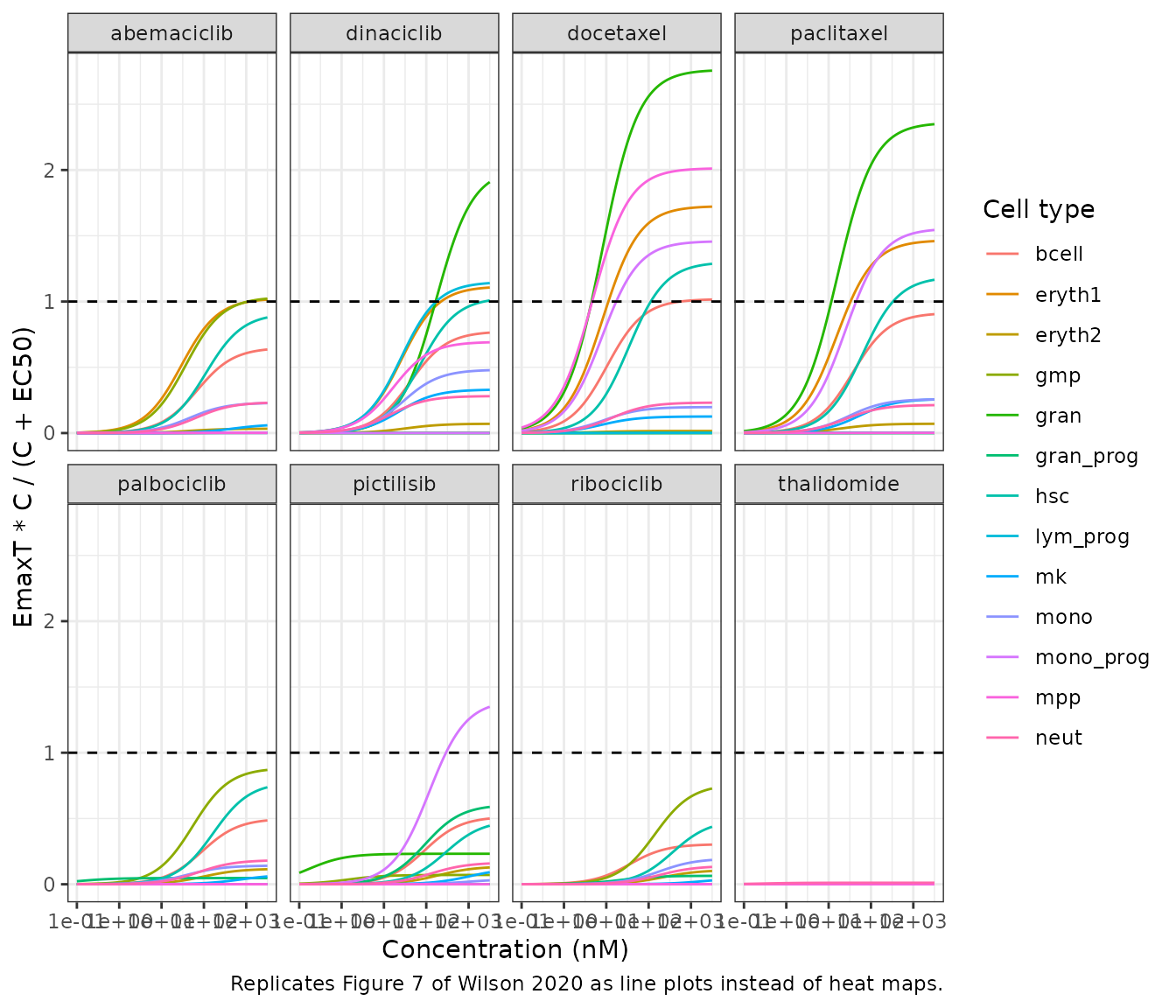
As in the paper, docetaxel, paclitaxel and dinaciclib reach effects above 1 (cell killing). All three kill HSC, granulocytes and early erythroid cells. Docetaxel also kills MPP, both taxanes kill monocyte progenitors, and dinaciclib kills lymphoid progenitors. By contrast, palbociclib acts mainly on HSC and GMP and stays below 1 (anti-proliferation only).
Replicates Supplementary Figures S1-S8: day-6 concentration-response
Each compound is simulated at the seven tested concentrations and at zero. Each day-6 count is divided by the drug-free day-6 count, which matches the normalization of the assay data to vehicle-control wells.
obs <- read.csv(text = "
drug,dose,HSCs,MPPs,GMPs,GranPs,Gran,MonoPs,Mon,Neut,ErythI,ErythII,MK,LymP,Blin,total_live,total_dead
abemaciclib,0.2,0.893,1.016,0.897,0.951,1.014,0.987,0.929,0.995,1.065,0.962,1.082,0.935,0.839,0.991,0.920
abemaciclib,1,1.030,0.983,1.077,1.003,1.074,0.994,1.094,1.000,1.158,1.120,0.995,0.994,1.035,1.082,0.976
abemaciclib,5,0.984,0.803,0.936,0.866,0.913,0.806,0.870,0.867,0.978,1.060,1.006,0.929,0.839,0.960,0.871
abemaciclib,25,0.667,0.443,0.504,0.520,0.346,0.275,0.418,0.308,0.471,0.579,0.842,0.389,0.508,0.477,0.468
abemaciclib,100,0.259,0.248,0.292,0.248,0.091,0.082,0.109,0.040,0.201,0.204,0.441,0.221,0.235,0.174,0.309
abemaciclib,500,0.053,0.276,0.058,0.024,0.020,0.016,0.037,0.003,0.048,0.018,0.084,0.223,0.041,0.031,0.220
abemaciclib,2500,0.027,0.036,0.006,0.000,0.001,0.001,0.006,0.000,0.006,0.000,0.006,0.075,0.001,0.003,0.340
dinaciclib,0.2,0.895,0.941,0.870,0.973,0.968,0.965,0.907,0.838,1.120,0.900,0.903,0.894,0.818,0.954,1.077
dinaciclib,1,1.063,1.036,1.106,0.997,1.205,1.056,1.055,0.831,1.043,1.076,1.107,1.052,0.904,1.074,1.056
dinaciclib,5,1.155,0.967,0.876,0.938,1.207,1.249,0.695,0.249,0.733,0.987,0.718,0.993,0.904,0.924,0.789
dinaciclib,25,0.612,0.534,0.403,0.317,0.328,0.618,0.086,0.007,0.239,0.232,0.118,0.383,0.117,0.261,0.348
dinaciclib,100,0.019,0.027,0.008,0.000,0.000,0.001,0.005,0.000,0.008,0.000,0.003,0.031,0.001,0.003,0.387
dinaciclib,500,0.052,0.027,0.017,0.000,0.001,0.002,0.008,0.000,0.009,0.000,0.005,0.078,0.005,0.004,0.341
dinaciclib,2500,0.013,0.009,0.007,0.000,0.000,0.002,0.005,0.000,0.008,0.000,0.004,0.025,0.001,0.003,0.396
docetaxel,0.2,0.979,0.910,1.025,1.102,0.997,1.095,1.031,0.908,1.118,0.916,0.947,0.964,0.890,1.003,1.041
docetaxel,1,1.041,1.069,1.257,1.095,1.116,1.075,1.062,0.996,1.100,1.045,1.094,1.308,0.948,1.082,1.070
docetaxel,5,0.646,0.639,0.152,0.046,0.021,0.077,0.026,0.002,0.053,0.004,0.144,0.243,0.035,0.047,1.133
docetaxel,25,0.040,0.024,0.004,0.000,0.000,0.002,0.012,0.002,0.006,0.000,0.011,0.060,0.002,0.003,0.457
docetaxel,100,0.005,0.007,0.002,0.000,0.000,0.002,0.011,0.001,0.004,0.000,0.007,0.027,0.015,0.002,0.461
docetaxel,500,0.023,0.020,0.007,0.000,0.001,0.003,0.020,0.001,0.007,0.000,0.010,0.077,0.013,0.004,0.416
docetaxel,2500,0.006,0.008,0.002,0.000,0.000,0.003,0.014,0.000,0.004,0.000,0.010,0.062,0.002,0.003,0.484
paclitaxel,0.2,1.085,0.787,1.265,1.139,1.040,1.023,0.909,0.883,1.242,0.909,1.081,1.215,1.018,1.020,1.052
paclitaxel,1,0.875,0.900,1.193,1.116,1.215,1.117,0.938,0.801,1.122,1.075,1.099,1.430,1.095,1.096,1.126
paclitaxel,5,1.179,0.713,1.091,1.061,0.928,0.890,0.770,0.523,0.835,0.565,1.114,0.613,0.759,0.759,1.146
paclitaxel,25,0.281,0.280,0.033,0.002,0.001,0.006,0.006,0.000,0.029,0.001,0.096,0.095,0.013,0.012,0.755
paclitaxel,100,0.048,0.023,0.001,0.000,0.001,0.001,0.004,0.000,0.004,0.000,0.010,0.054,0.002,0.002,0.475
paclitaxel,500,0.011,0.006,0.007,0.000,0.000,0.002,0.010,0.000,0.006,0.000,0.008,0.073,0.004,0.003,0.407
paclitaxel,2500,0.013,0.004,0.003,0.000,0.000,0.003,0.003,0.000,0.004,0.000,0.008,0.096,0.003,0.002,0.461
palbociclib,0.2,0.894,0.864,0.923,0.982,0.947,1.014,0.900,0.951,1.042,0.890,0.860,0.861,0.934,0.948,1.009
palbociclib,1,0.920,0.884,0.942,1.070,0.939,0.923,1.059,0.938,1.087,1.028,0.966,0.880,1.055,0.996,1.018
palbociclib,5,0.985,0.773,0.925,0.918,0.882,0.973,0.899,0.746,0.964,0.991,0.891,0.731,0.766,0.918,1.026
palbociclib,25,0.834,0.456,0.763,0.734,0.539,0.444,0.588,0.517,0.721,0.823,0.912,0.380,0.673,0.698,0.646
palbociclib,100,0.489,0.233,0.539,0.370,0.215,0.141,0.256,0.211,0.351,0.569,0.622,0.124,0.414,0.396,0.405
palbociclib,500,0.250,0.110,0.239,0.080,0.046,0.046,0.132,0.039,0.094,0.303,0.236,0.052,0.138,0.154,0.289
palbociclib,2500,0.099,0.058,0.046,0.008,0.004,0.008,0.239,0.007,0.023,0.143,0.079,0.046,0.088,0.061,0.227
pictilisib,0.2,0.891,0.893,0.956,0.955,0.992,1.051,0.925,0.927,1.102,0.946,1.001,0.933,0.938,0.978,1.051
pictilisib,1,1.023,0.822,0.979,1.000,1.002,0.943,0.906,0.826,1.068,0.920,1.074,1.050,1.075,0.964,1.100
pictilisib,5,0.885,0.717,0.927,1.015,0.903,0.872,0.795,0.645,1.069,0.900,1.129,0.869,0.815,0.912,0.915
pictilisib,25,0.992,0.672,0.754,0.840,0.786,0.748,0.776,0.598,1.000,0.867,0.856,0.777,0.655,0.840,0.931
pictilisib,100,0.581,0.491,0.625,0.702,0.514,0.490,0.611,0.304,0.928,0.555,0.784,0.496,0.375,0.601,0.553
pictilisib,500,0.281,0.382,0.395,0.608,0.279,0.302,0.309,0.062,0.655,0.233,0.497,0.464,0.162,0.339,0.401
pictilisib,2500,0.081,0.280,0.225,0.284,0.098,0.113,0.125,0.005,0.275,0.059,0.168,0.192,0.062,0.129,0.343
ribociclib,0.2,0.903,0.814,0.912,0.871,0.929,1.004,0.843,0.772,1.012,0.843,1.018,0.878,0.743,0.900,1.166
ribociclib,1,0.939,0.919,0.925,1.048,0.981,1.084,0.967,0.831,1.025,0.977,0.983,0.952,1.075,0.978,1.170
ribociclib,5,1.067,0.838,1.030,1.043,1.091,0.998,0.921,0.964,1.083,1.130,0.917,1.003,0.794,1.060,1.290
ribociclib,25,0.987,0.637,0.850,0.813,0.746,0.802,0.781,0.654,0.858,0.814,0.836,0.617,0.612,0.794,0.811
ribociclib,100,0.894,0.469,0.734,0.703,0.507,0.456,0.554,0.527,0.690,0.798,1.013,0.391,0.463,0.666,0.600
ribociclib,500,0.677,0.284,0.544,0.344,0.237,0.167,0.314,0.251,0.312,0.667,0.644,0.174,0.280,0.421,0.321
ribociclib,2500,0.352,0.169,0.295,0.108,0.067,0.070,0.085,0.048,0.094,0.336,0.277,0.043,0.283,0.178,0.278
thalidomide,0.2,0.676,0.918,0.924,0.809,0.850,0.901,0.833,0.995,1.006,0.943,0.978,1.092,0.908,0.908,0.916
thalidomide,1,0.926,0.759,1.070,0.972,1.001,0.935,0.940,0.791,1.198,0.998,1.032,1.048,0.996,0.998,1.094
thalidomide,5,1.089,0.790,1.001,1.136,1.101,0.984,0.894,0.882,1.242,1.048,1.175,1.233,1.077,1.080,0.963
thalidomide,25,0.963,0.875,1.120,1.304,1.256,1.196,1.057,0.945,1.224,1.109,1.140,1.260,1.155,1.159,1.196
thalidomide,100,0.849,0.767,0.970,0.990,0.949,0.920,0.944,0.624,1.367,0.778,1.015,0.946,0.930,0.931,1.125
thalidomide,500,0.998,0.781,1.043,0.945,0.927,0.827,0.999,0.690,1.136,0.875,0.881,0.766,0.915,0.917,1.047
thalidomide,2500,1.132,0.915,0.990,1.089,1.022,1.039,0.973,0.969,1.363,0.937,1.045,1.395,1.036,1.037,0.998
", check.names = FALSE)
obsCols <- c(HSCs = "hsc", MPPs = "mpp", GMPs = "gmp", GranPs = "gran_prog",
             Gran = "gran", MonoPs = "mono_prog", Mon = "mono", Neut = "neut",
             ErythI = "eryth1", ErythII = "eryth2", MK = "mk", LymP = "lym_prog",
             Blin = "bcell", total_live = "totalViableCells",
             total_dead = "dead_cells")
simDay6 <- function(drug, conc) {
  ev <- et(amt = conc, cmt = "drug", time = 0) |> et(6)
  s <- as.data.frame(rxSolve(ui, ev, params = drugPar[[drug]]))
  s[s$time == 6, unname(obsCols)]
}
ctl6 <- simDay6("docetaxel", 0)
simResp <- expand.grid(drug = refDrugs, dose = concs, stringsAsFactors = FALSE)
simResp <- bind_cols(simResp, do.call(rbind, Map(simDay6, simResp$drug, simResp$dose)))
simResp[unname(obsCols)] <- sweep(as.matrix(simResp[unname(obsCols)]), 2,
                                   as.numeric(ctl6), "/")
names(simResp) <- c("drug", "dose", names(obsCols))
gof <- inner_join(
  pivot_longer(obs, -c(drug, dose), names_to = "cell", values_to = "observed"),
  pivot_longer(simResp, -c(drug, dose), names_to = "cell", values_to = "simulated"),
  by = c("drug", "dose", "cell")
)
stopifnot(nrow(gof) == 8 * 7 * 15)
ggplot(gof, aes(dose)) +
  geom_point(aes(y = observed), shape = 1) +
  geom_line(aes(y = simulated, colour = drug)) +
  scale_x_log10() +
  facet_grid(cell ~ drug) +
  labs(x = "Concentration (nM)", y = "Day-6 count / vehicle control",
       caption = "Replicates Supplementary Figures S1-S8 of Wilson 2020 (circles: S1 Table; lines: model).") +
  theme_bw(base_size = 7) +
  theme(legend.position = "none")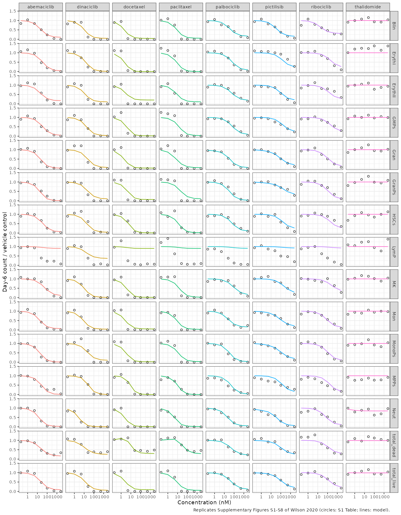
Mean squared error per compound, with the paper’s lymphoid-progenitor column shown separately (see Assumptions and deviations):
mseTab <- gof |>
  mutate(group = ifelse(cell == "LymP", "LymP", "other")) |>
  group_by(drug, group) |>
  summarise(mse = mean((observed - simulated)^2),
            medAbs = median(abs(observed - simulated)), .groups = "drop") |>
  pivot_wider(names_from = group, values_from = c(mse, medAbs))
mseTab |>
  mutate(across(where(is.numeric), \(x) round(x, 3))) |>
  rename(
    "Compound" = drug,
    "MSE, lymphoid progenitors" = mse_LymP,
    "MSE, other 14 outputs" = mse_other,
    "Median |obs - sim|, lymphoid progenitors" = medAbs_LymP,
    "Median |obs - sim|, other 14 outputs" = medAbs_other
  ) |>
knitr::kable()| Compound | MSE, lymphoid progenitors | MSE, other 14 outputs | Median |obs - sim|, lymphoid progenitors | Median |obs - sim|, other 14 outputs |
|---|---|---|---|---|
| abemaciclib | 0.284 | 0.007 | 0.571 | 0.056 |
| dinaciclib | 0.069 | 0.017 | 0.230 | 0.094 |
| docetaxel | 0.495 | 0.029 | 0.825 | 0.076 |
| paclitaxel | 0.450 | 0.026 | 0.807 | 0.089 |
| palbociclib | 0.373 | 0.005 | 0.593 | 0.053 |
| pictilisib | 0.151 | 0.008 | 0.212 | 0.060 |
| ribociclib | 0.267 | 0.012 | 0.374 | 0.070 |
| thalidomide | 0.049 | 0.018 | 0.233 | 0.081 |
# Deterministic simulation of the paper's own fitted parameters against its
# own fitting data: a mis-transcribed flux, stoichiometry or parameter moves
# these errors by far more than the margins below.
stopifnot(
  all(mseTab$medAbs_other < 0.12),
  all(mseTab$mse_other < 0.04)
)
Outside the lymphoid progenitors, the model reproduces the assay data with a median absolute error below 0.1 on the vehicle-normalized scale for every reference compound, including the thalidomide negative control. The mean squared errors are largest for docetaxel and paclitaxel, the two compounds with the strongest cell-killing effects.
Drug-free sanity check
With every EmaxT at zero, the drug state has no effect at any concentration:
simHigh <- as.data.frame(rxSolve(ui, et(amt = 2500, cmt = "drug", time = 0) |> et(6)))
simZero <- as.data.frame(rxSolve(ui, et(amt = 0, cmt = "drug", time = 0) |> et(6)))
stopifnot(isTRUE(all.equal(simHigh$totalViableCells, simZero$totalViableCells)),
          isTRUE(all.equal(simHigh$dead_cells, simZero$dead_cells)))
NCA
Non-compartmental analysis does not apply. The model has no pharmacokinetics: the in vitro drug concentration is constant for the whole culture, and every output is a cell count. The quantitative validation here is the concentration-response comparison above against the paper’s own fitting data (S1 Table).
Assumptions and deviations
-
Neutrophil split at t = 0. S1 Text splits the
neutrophils into quiescent and proliferating pools with an event at t =
0.01 day. The packaged model applies the split as an initial condition.
The exact event is reproduced above with
evid = 5. Day-6 neutrophils differ by about 2%, and no upstream cell type changes. - Lymphoid progenitors were not part of the drug-effect fit. The Methods list of cell types fitted in the drug-effect step (“hematopoietic stem cells … and B cells (B-lin)”) and the rows of Figure 4 both omit lymphoid progenitors, although S2 Table carries an EmaxT and EC50 for them. The Methods text says 13 cell types but lists only 12. The assay’s lymphoid-progenitor counts fall with concentration for most compounds, but the fitted EmaxT for this cell type is near zero for all reference compounds except dinaciclib, so the model barely moves. This matches the model as published, not a transcription error, and the lymphoid-progenitor misfit is reported separately above.
-
renewal_Monois not carried. S1 Text listsrenewal_Mono = 0.26505, but no flux uses it (monocyte-lineage cells are terminal and proliferate without renewal), so it has no effect on the model. -
Named compounds only. S2 Table has drug-effect
parameters for 51 compounds, 37 of them anonymized development compounds
(
class2_drug1,Pi3K_drug4, …). The 14 named compounds are carried indrugEffectParameters; 5-FU is keyed asfluorouracil. Values come from the sheet of fitted natural-log EC50s. The sheet of EC50s is its exponential and agrees with Table 1. -
Drug-free defaults.
lec50_* = 1is the SimBiology default and has no effect whileemaxt_* = 0. It is not an estimate. - No variability. The paper fitted donor-mean data by a genetic algorithm with local search and reports no between-donor variability or residual error, so none is encoded.
-
Units. SimBiology counts cells as
moleculein a 1 mL compartment. The states are therefore cells/mL, the unit of Figure 3. The drug state is a concentration in nM (the unit of EC50), set by a bolus withamt= concentration.