Prostate cancer signaling logic-based ODE network (Traynard 2017)
Source:vignettes/articles/Traynard_2017_prostateSignaling_qsp.Rmd
Traynard_2017_prostateSignaling_qsp.RmdModel and source
- Citation: Traynard P, Tobalina L, Eduati F, Calzone L, Saez-Rodriguez J (2017). Logic Modeling in Quantitative Systems Pharmacology. CPT Pharmacometrics Syst Pharmacol 6(8):499-511. doi:10.1002/psp4.12225. PMCID: PMC5572374. The trained model is published only in the supplementary GitHub repository https://github.com/saezlab/CPT_QSPtutorial (GPLv3), cited in the paper’s Supplementary Materials section; the main text prints the structural ODE form and two of the 25 edge strengths. Node lifetimes tau are supplement file logicODEparameters_nodes.txt; edge strengths k are supplement file logicODEparameters_edges.txt; the prior knowledge network is supplement file PriorKnowledgeNetwork.sif; the fitting script is supplement file CellNOptR_optimisation.R. Training data: Lescarbeau RM, Kaplan DL (2014). Quantitative analysis of castration resistant prostate cancer progression through phosphoproteome signaling. BMC Cancer 14:325. doi:10.1186/1471-2407-14-325. Transfer-function and right-hand-side definitions were read from the C sources of CNORode2017 (github.com/saezlab/CNORode2017), the package the supplement’s fitting script installs and calls.
- Description: QSP. In vitro (LNCaP human prostate cancer cell line). Logic-based ODE model of the MAPK / PI3K / JAK-STAT / IKK signaling network that drives castration-resistant prostate cancer survival (Traynard 2017, the worked example of a CPT:PSP logic-modeling tutorial). Twenty network nodes are carried as ODE states holding a normalized activity on [0, 1]; five ligand stimuli (EGF, IGF-1, IL-6, TNF-alpha, DHT) and five kinase inhibitors (PI3K, MEK, mTOR, p38, IKK) enter as per-condition covariates. Each state relaxes toward the continuous (HillCube) homologue of its Boolean rule at a node-specific rate tau, with each regulatory edge passed through a normalized Hill transfer function of strength k. Multi-input nodes (AR, PI3K, RAS, JNK) use continuous OR. The 45 estimated parameters (20 tau, 25 k) were fitted with CellNOptR / CNORode2017 to 44 perturbation conditions of the Lescarbeau 2014 LNCaP phosphoproteome data at 30 and 240 min. All activities start at the normalized basal value 0.5; a fully inhibited node is held at basal. Deterministic: no IIV and no residual error are reported. The paper’s companion MaBoSS continuous-time Boolean model (which adds the Survival, Cell_cycle, MYC, Caspase8, Caspase9, p53, NFkB and beta-catenin nodes) is a stochastic Markov process over Boolean states, not an ODE system, and is therefore not part of this file.
- Article: https://doi.org/10.1002/psp4.12225 (PMCID: PMC5572374, open access)
- Supplementary materials (model files, fitted parameters, training data, fitting script): https://github.com/saezlab/CPT_QSPtutorial (GPLv3)
- Training data source: Lescarbeau RM, Kaplan DL (2014) BMC Cancer 14:325, https://doi.org/10.1186/1471-2407-14-325
Traynard 2017 is a CPT:PSP tutorial on logic
modeling, but its worked example is a real model fitted to real
published data: a 20-node logic-based ODE network of prostate cancer
signaling, trained with CellNOptR /
CNORode2017 against 44 perturbation conditions of the
Lescarbeau 2014 LNCaP phosphoproteome dataset. The 45 fitted parameters
(20 node lifetimes tau, 25 edge strengths k)
are published in the supplementary repository, so the model is
reproducible end to end. That is what this file packages.
The paper’s other model – a continuous-time Boolean (MaBoSS)
Markov process over the full, uncompressed network including a
Survival phenotype node – is a stochastic process over
Boolean states rather than an ODE system and is not packaged here. See
Assumptions and deviations below.
Population
The “subject” in this model is a perturbation condition, not an organism. The system is the LNCaP human prostate cancer cell line, an androgen-sensitive line used to study the transition to castration-resistant growth.
Lescarbeau 2014 perturbed LNCaP cells with combinations of five ligands (EGF, IGF-1, IL-6, TNF-alpha and the androgen DHT) and five kinase inhibitors (PI3K, MEK, IKK, mTOR and p38), giving 44 conditions, and assayed eight phosphosites (AKT, RPS6, GSK3, ERK1/2, p38, JNK, HSP27, Stat3) at 30 min, 4 h and 24 h with an antibody-based panel. Traynard 2017 used the 30 min and 4 h timepoints only, reasoning that phosphorylation signaling reaches a semi-steady state within a few hours while a 24 h window would require modeling transcriptional rewiring. The docetaxel arm of Lescarbeau 2014 was excluded because it produced little phosphoproteome variation and its target (beta-tubulin) lies outside the network.
Measurements were normalized per phosphosite as the log2 fold change
versus the unperturbed basal state and then linearly rescaled onto
[0, 1] with 0.5 at basal. Every model
state therefore starts at 0.5, and an unstimulated ligand input node is
also held at 0.5 rather than 0.
The same information is available programmatically:
readModelDb("Traynard_2017_prostateSignaling_qsp")()$population[
  c("species", "n_subjects", "n_conditions", "n_measured_nodes", "disease_state")
]
#> $species
#> [1] "in vitro (LNCaP human prostate cancer cell line)"
#>
#> $n_subjects
#> [1] 44
#>
#> $n_conditions
#> [1] 44
#>
#> $n_measured_nodes
#> [1] 8
#>
#> $disease_state
#> [1] "castration-resistant prostate cancer (LNCaP, an androgen-sensitive line used to study the transition to androgen independence)"
Model structure
Each network node j carries a normalized activity on
[0, 1] and relaxes toward the continuous homologue of its
Boolean rule:
-
tau_jis the node lifetime parameter.tau_j = 0freezes the node at its initial (basal) value – Traynard 2017 states this explicitly for IGF1_R, TNFR and IKK. -
fis the edge transfer function. The supplement’s fitting script selectstransfer_function = 4, whichCNORode2017dispatches toFG_transfer_function(): a monotone sigmoid withf(0) = 0,f(1) = 1, andfidentically zero whenk = 0(the paper’s “when k = 0 the dynamic of AKT is independent from PI3K”). The Hill exponentnwas held at the CNORode default of 3 (opt_n = FALSE). -
B_jis the multilinear (HillCube) homologue of nodej’s Boolean rule. All four multi-input nodes in the trained model (AR, PI3K, RAS, JNK) are OR gates, whose homologue is1 - prod(1 - f_i). -
inh_jis the inhibitor covariate for that node; a fully inhibited node has a zero derivative and so is pinned at the basal value 0.5.
mod <- rxode2::rxode2(readModelDb("Traynard_2017_prostateSignaling_qsp"))
rxode2::rxState(mod)
#>  [1] "EGFR"   "IGF1_R" "IL6R"   "TNFR"   "AR"     "PI3K"   "AKT"    "mTOR"
#>  [9] "RPS6"   "GSK3a"  "Jak"    "Stat3"  "RAS"    "MEK"    "ERK1_2" "Rac"
#> [17] "p38"    "HSP27"  "JNK"    "IKKa"
Source trace
Values that are not in the article PDF come from the supplementary GitHub repository the article’s Supplementary Materials section points to. Every file named below is in that repository.
| Item | Source |
|---|---|
ODE right-hand side
tau * (B - x) * (1 - inh)
|
Article, ‘Training the logic-based ODE model with
CellNOpt’ (AKT instance printed in text); general form CNORode2017
src/rhsODE.c
|
| Transfer function f(x, n, k) |
transferFun = 4 in supplement
CellNOptR_optimisation.R; dispatched to
FG_transfer_function in CNORode2017
src/sim_logic_ode.c, defined in
src/FG_transfer_function.c
|
| Hill exponent n = 3, not estimated | Supplement CellNOptR_optimisation.R:
createLBodeContPars(..., default_n = 3, opt_n = FALSE)
|
| OR gate for multi-input nodes | Article Figure 2b caption: ‘All other nodes in the model with more than one input edge are modeled with a simple OR gate’ |
| Network topology (20 states, 25 edges) | Supplement PriorKnowledgeNetwork.sif after
CellNOptR compression; independently confirmed by supplement
trainedmodel.bnd and Article Figure 3a |
| 20 node lifetimes tau | Supplement logicODEparameters_nodes.txt;
independently reproduced as $u_<node> in supplement
trainedmodel.cfg
|
| 25 edge strengths k | Supplement
logicODEparameters_edges.txt
|
| k(Rac -> JNK) = 6.7e-05, k(AKT -> AR) = 8.4e-04 | Printed in the article main text, section ‘Simulation of a logical model in different conditions’ |
| tau(IGF1_R) = tau(TNFR) = tau(IKKa) = 0 | Supplement logicODEparameters_nodes.txt;
stated in the article text after Table 1 and shown as white boxes in
Figure 3a |
| Initial condition 0.5 for every state | Article, normalization step 3: ‘all initial conditions
are set to 0.5 (which is the basal state…)’; CNORode2017
src/simulateODE.c sets the whole state array to 0.5 |
| Unstimulated stimulus node = 0.5 | Supplement CellNOptR_optimisation.R:
cnolist$valueStimuli[cnolist$valueStimuli==0]=0.5
|
| Inhibitor pins its node at the initial value | CNORode2017 src/rhsODE.c: the whole
derivative is multiplied by (1 - inhibitor_array[j])
|
| Training data (44 conditions x 2 timepoints x 8 phosphosites) | Supplement
perturbationData_LNCaP_MIDAS.csv, shipped here as
inst/extdata/Traynard_2017_perturbationData_LNCaP_MIDAS.csv
|
| Validation targets r = 0.66 and MSE = 0.017 | Article Figure 3c annotation |
Experimental design and simulation
The MIDAS training file is shipped with the package. The design
matrix is recovered from its TR: columns, recoding an
absent stimulus to the normalized basal value 0.5 exactly as the
supplement’s fitting script does.
midas_path <- system.file(
  "extdata", "Traynard_2017_perturbationData_LNCaP_MIDAS.csv",
  package = "nlmixr2lib"
)
stopifnot(nzchar(midas_path))

midas <- read.csv(midas_path, check.names = FALSE)
names(midas) <- gsub(":", "_", sub("^TR:", "TR_", sub("^DV:", "DV_", sub("^DA:", "DA_", names(midas)))))

design <-
  midas |>
  dplyr::filter(DA_ALL == 0) |>
  dplyr::transmute(
    id = dplyr::row_number(),
    STIM_EGF_NORM = ifelse(TR_EGF == 1, 1, 0.5),
    STIM_IGF1_NORM = ifelse(TR_IGF_1 == 1, 1, 0.5),
    STIM_IL6_NORM = ifelse(TR_IL6 == 1, 1, 0.5),
    STIM_TNFA_NORM = ifelse(TR_TNFa == 1, 1, 0.5),
    STIM_DHT_NORM = ifelse(TR_DHT == 1, 1, 0.5),
    PI3K_INHIBITED = TR_PI3Ki,
    MEK_INHIBITED = TR_MEKi,
    MTOR_INHIBITED = TR_mTORi,
    P38_INHIBITED = TR_p38i,
    IKK_INHIBITED = TR_IKKai
  )

stopifnot(nrow(design) == 44L)
knitr::kable(
  head(design, 8),
  caption = "First eight of the 44 perturbation conditions (0.5 = ligand absent)."
)| id | STIM_EGF_NORM | STIM_IGF1_NORM | STIM_IL6_NORM | STIM_TNFA_NORM | STIM_DHT_NORM | PI3K_INHIBITED | MEK_INHIBITED | MTOR_INHIBITED | P38_INHIBITED | IKK_INHIBITED |
|---|---|---|---|---|---|---|---|---|---|---|
| 1 | 0.5 | 0.5 | 0.5 | 0.5 | 0.5 | 0 | 0 | 0 | 0 | 0 |
| 2 | 1.0 | 0.5 | 0.5 | 0.5 | 0.5 | 0 | 0 | 0 | 0 | 0 |
| 3 | 0.5 | 1.0 | 0.5 | 0.5 | 0.5 | 0 | 0 | 0 | 0 | 0 |
| 4 | 0.5 | 0.5 | 1.0 | 0.5 | 0.5 | 0 | 0 | 0 | 0 | 0 |
| 5 | 0.5 | 0.5 | 0.5 | 1.0 | 0.5 | 0 | 0 | 0 | 0 | 0 |
| 6 | 0.5 | 0.5 | 0.5 | 0.5 | 1.0 | 0 | 0 | 0 | 0 | 0 |
| 7 | 1.0 | 0.5 | 0.5 | 0.5 | 0.5 | 1 | 0 | 0 | 0 | 0 |
| 8 | 0.5 | 1.0 | 0.5 | 0.5 | 0.5 | 1 | 0 | 0 | 0 | 0 |
The model is deterministic – Traynard 2017 reports no between-subject variability and no residual error – so a single solve per condition is the whole cohort. 44 conditions is well inside the 200-per-arm vignette cap.
measured <- c("AKT", "RPS6", "GSK3a", "ERK1_2", "p38", "JNK", "HSP27", "Stat3")

ev_fit <- merge(design["id"], as.data.frame(rxode2::et(c(0, 30, 240))), by = NULL)
ev_fit <- dplyr::arrange(ev_fit, id, time)

sim_fit <- rxode2::rxSolve(mod, events = ev_fit, params = design, returnType = "data.frame")

obs_long <-
  midas |>
  dplyr::filter(DA_ALL > 0) |>
  dplyr::mutate(id = rep(seq_len(44), times = 2L)) |>
  dplyr::select(id, time = DA_ALL, dplyr::all_of(paste0("DV_", measured))) |>
  tidyr::pivot_longer(-c(id, time), names_to = "node", values_to = "observed") |>
  dplyr::mutate(node = sub("^DV_", "", node))

pred_long <-
  sim_fit |>
  dplyr::select(id, time, dplyr::all_of(measured)) |>
  tidyr::pivot_longer(-c(id, time), names_to = "node", values_to = "predicted")

fit <- dplyr::inner_join(obs_long, pred_long, by = c("id", "time", "node"))
stopifnot(nrow(fit) == 44L * 2L * 8L, !anyNA(fit$observed), !anyNA(fit$predicted))
Replicating Figure 3c: goodness of fit against the published metrics
Figure 3c of Traynard 2017 plots simulated against measured normalized values over all 704 training observations and annotates the panel with two numbers: Pearson correlation = 0.66 and MSE = RSS/N = 0.017. Those are printed values, so they are an exact answer key for the whole transcription – the 45 parameters, the transfer function, the OR gates, the inhibitor semantics, the initial conditions and the stimulus recoding all have to be right simultaneously for them to come out.
pearson_r <- cor(fit$observed, fit$predicted)
mse <- mean((fit$observed - fit$predicted)^2)
cod <- 1 - sum((fit$observed - fit$predicted)^2) / sum((fit$observed - mean(fit$observed))^2)

knitr::kable(
  tibble::tibble(
    Metric = c("Pearson correlation r", "MSE = RSS/N", "Coefficient of determination"),
    Published = c("0.66", "0.017", "(shown graphically only, Figure 3d)"),
    Reproduced = c(sprintf("%.4f", pearson_r), sprintf("%.5f", mse), sprintf("%.4f", cod))
  ),
  caption = "Figure 3c annotations versus this package's solve of the same model."
)| Metric | Published | Reproduced |
|---|---|---|
| Pearson correlation r | 0.66 | 0.6579 |
| MSE = RSS/N | 0.017 | 0.01727 |
| Coefficient of determination | (shown graphically only, Figure 3d) | 0.4269 |
# These are printed point values compared against a fully deterministic solve --
# no random cohort is involved, so the only difference that can arise is ODE
# solver tolerance. A tight bound is the correct assertion here.
stopifnot(
  abs(round(pearson_r, 2) - 0.66) < 1e-8,
  abs(round(mse, 3) - 0.017) < 1e-8
)
ggplot2::ggplot(fit, ggplot2::aes(observed, predicted)) +
  ggplot2::geom_hline(yintercept = 0.5, linetype = "dashed", colour = "grey60") +
  ggplot2::geom_vline(xintercept = 0.5, linetype = "dashed", colour = "grey60") +
  ggplot2::geom_point(size = 0.8, alpha = 0.6) +
  ggplot2::geom_smooth(method = "lm", formula = y ~ x, colour = "grey40", se = TRUE) +
  ggplot2::coord_cartesian(xlim = c(0, 1), ylim = c(0, 1)) +
  ggplot2::labs(
    x = "normalised measured values", y = "model simulation",
    subtitle = sprintf("Pearson correlation = %.2f; MSE = RSS/N = %.3f", pearson_r, mse)
  ) +
  ggplot2::theme_bw()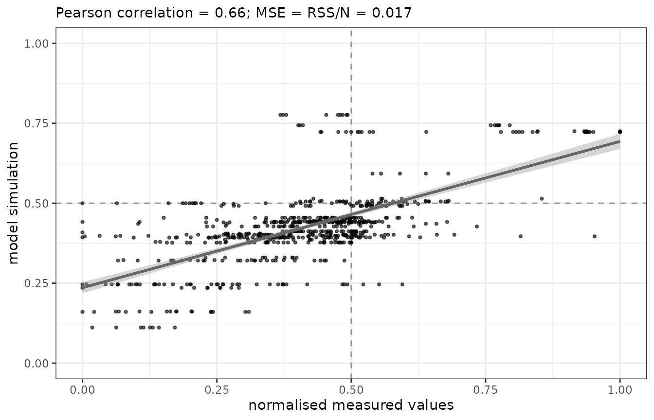
Replicates Figure 3c of Traynard 2017: model simulation versus normalised measured values over all 44 conditions, 2 timepoints and 8 phosphosites.
Replicating Figure 3b: per-condition fitting-error heatmap
Figure 3b shows the mean squared error of each measured phosphoprotein in each experimental condition on a white-to-dark-orange scale capped at 0.25, above a green/red grid of the experimental design. The same quantity is reproduced here.
err <-
  fit |>
  dplyr::group_by(id, node) |>
  dplyr::summarise(mse = mean((observed - predicted)^2), .groups = "drop") |>
  dplyr::mutate(node = factor(node, levels = rev(c("HSP27", "ERK1_2", "Stat3", "p38", "AKT", "RPS6", "GSK3a", "JNK"))))

design_long <-
  design |>
  dplyr::mutate(
    EGF = STIM_EGF_NORM == 1, IGF_1 = STIM_IGF1_NORM == 1, IL6 = STIM_IL6_NORM == 1,
    TNFa = STIM_TNFA_NORM == 1, DHT = STIM_DHT_NORM == 1,
    `PI3K i` = PI3K_INHIBITED == 1, `IKK i` = IKK_INHIBITED == 1, `MEK i` = MEK_INHIBITED == 1,
    `mTOR i` = MTOR_INHIBITED == 1, `p38 i` = P38_INHIBITED == 1
  ) |>
  dplyr::select(id, EGF, IGF_1, IL6, TNFa, DHT, `PI3K i`, `IKK i`, `MEK i`, `mTOR i`, `p38 i`) |>
  tidyr::pivot_longer(-id, names_to = "row", values_to = "on") |>
  dplyr::mutate(
    kind = ifelse(row %in% c("EGF", "IGF_1", "IL6", "TNFa", "DHT"), "Stimulus", "Inhibitor"),
    row = factor(row, levels = rev(c("EGF", "IGF_1", "IL6", "TNFa", "DHT", "PI3K i", "IKK i", "MEK i", "mTOR i", "p38 i")))
  )

p_err <-
  ggplot2::ggplot(err, ggplot2::aes(factor(id), node, fill = pmin(mse, 0.25))) +
  ggplot2::geom_tile(colour = "grey85", linewidth = 0.1) +
  ggplot2::scale_fill_gradientn(
    colours = c("#FFFFF0", "#FEE08B", "#F46D43", "#8C2D04"), limits = c(0, 0.25),
    name = "Mean\nSquared\nError (MSE)"
  ) +
  ggplot2::labs(x = NULL, y = "Measured phosphoproteins") +
  ggplot2::theme_minimal() +
  ggplot2::theme(axis.text.x = ggplot2::element_blank(), panel.grid = ggplot2::element_blank())

p_des <-
  ggplot2::ggplot(design_long, ggplot2::aes(factor(id), row)) +
  ggplot2::geom_tile(ggplot2::aes(fill = ifelse(on, kind, NA_character_)), colour = "grey85", linewidth = 0.1) +
  ggplot2::scale_fill_manual(
    values = c(Stimulus = "#7CB342", Inhibitor = "#E53935"), na.value = "white",
    name = NULL, na.translate = FALSE
  ) +
  ggplot2::labs(x = "Experimental condition", y = "Experimental condition") +
  ggplot2::theme_minimal() +
  ggplot2::theme(axis.text.x = ggplot2::element_blank(), panel.grid = ggplot2::element_blank())

print(p_err)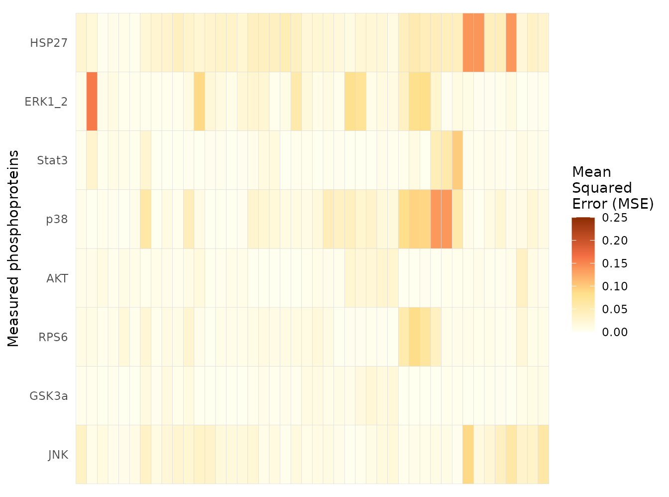
Replicates Figure 3b (lower panel) of Traynard 2017: per-condition, per-phosphoprotein fitting error, with the experimental design below.
print(p_des)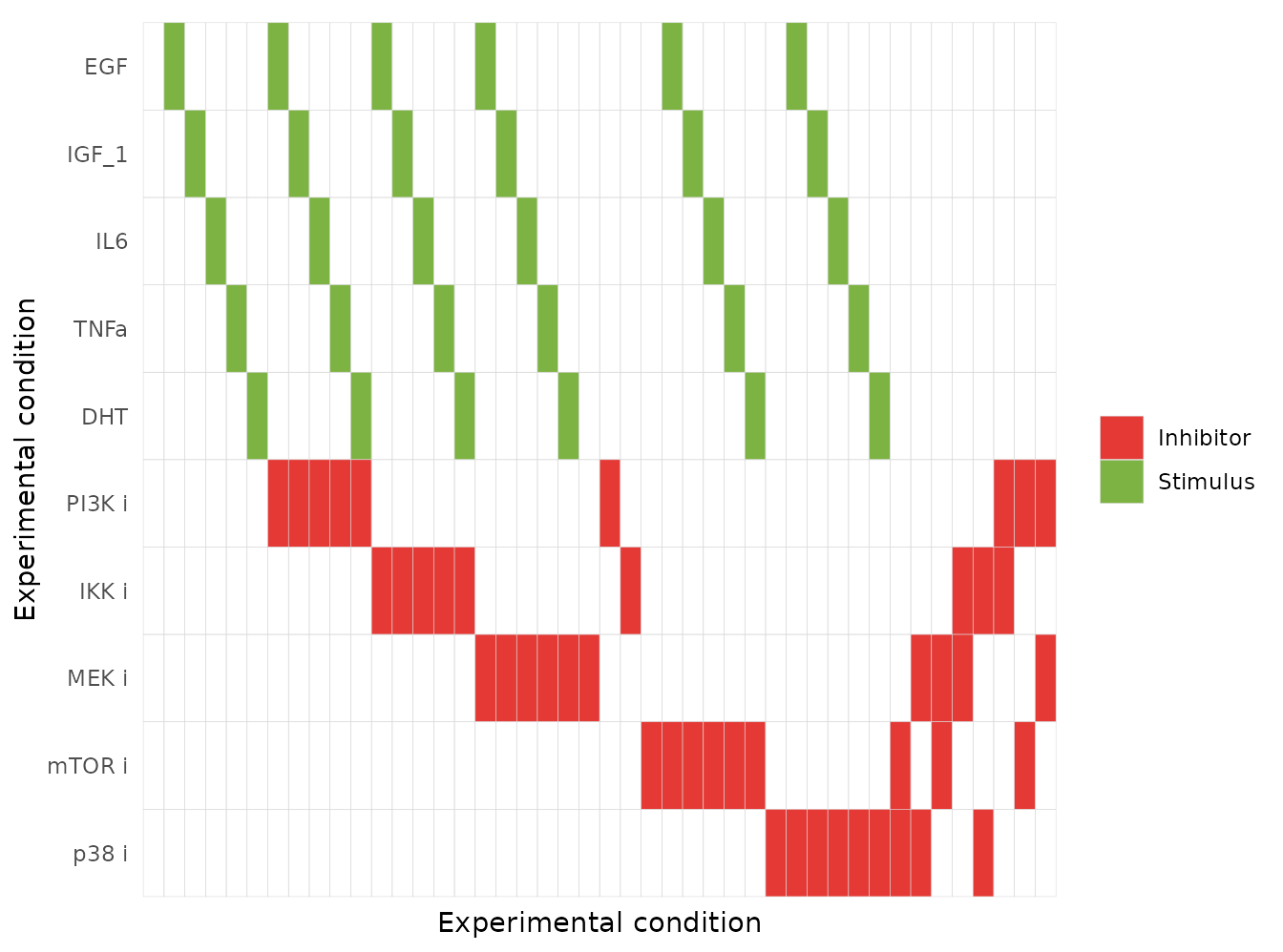
Replicates Figure 3b (lower panel) of Traynard 2017: per-condition, per-phosphoprotein fitting error, with the experimental design below.
As in the published panel, the fit is good for most conditions (the bulk of the heatmap is near-white) and the worst errors concentrate in a handful of inhibitor-containing conditions, notably for p38 and Stat3.
condition_label <-
  design |>
  dplyr::transmute(
    id = id,
    condition = trimws(paste0(
      ifelse(STIM_EGF_NORM == 1, "EGF ", ""), ifelse(STIM_IGF1_NORM == 1, "IGF1 ", ""),
      ifelse(STIM_IL6_NORM == 1, "IL6 ", ""), ifelse(STIM_TNFA_NORM == 1, "TNFa ", ""),
      ifelse(STIM_DHT_NORM == 1, "DHT ", ""), ifelse(PI3K_INHIBITED == 1, "+PI3Ki ", ""),
      ifelse(MEK_INHIBITED == 1, "+MEKi ", ""), ifelse(MTOR_INHIBITED == 1, "+mTORi ", ""),
      ifelse(P38_INHIBITED == 1, "+p38i ", ""), ifelse(IKK_INHIBITED == 1, "+IKKi ", "")
    ))
  ) |>
  dplyr::mutate(condition = ifelse(nzchar(condition), condition, "control"))

err |>
  dplyr::slice_max(mse, n = 6) |>
  dplyr::left_join(condition_label, by = "id") |>
  dplyr::transmute(Condition = condition, Phosphoprotein = as.character(node), MSE = round(mse, 3)) |>
knitr::kable(caption = "The six worst-fitting condition / phosphoprotein cells.")| Condition | Phosphoprotein | MSE |
|---|---|---|
| EGF | ERK1_2 | 0.158 |
| +mTORi +p38i | HSP27 | 0.139 |
| +MEKi +p38i | HSP27 | 0.139 |
| TNFa +p38i | p38 | 0.138 |
| +p38i +IKKi | HSP27 | 0.138 |
| IL6 +p38i | p38 | 0.138 |
Replicating Figure 3b (upper panels): example time courses
Figure 3b also shows four example fits of simulated activity against the measured points. The same comparison is drawn here for four representative conditions.
ev_dense <- merge(design["id"], as.data.frame(rxode2::et(seq(0, 240, by = 2))), by = NULL)
ev_dense <- dplyr::arrange(ev_dense, id, time)
sim_dense <- rxode2::rxSolve(mod, events = ev_dense, params = design, returnType = "data.frame")

examples <- tibble::tribble(
  ~id, ~node,
  which(design$STIM_EGF_NORM == 1 & rowSums(design[, c("PI3K_INHIBITED", "MEK_INHIBITED", "MTOR_INHIBITED", "P38_INHIBITED", "IKK_INHIBITED")]) == 0)[1], "ERK1_2",
  which(rowSums(design[, 2:6] == 1) == 0 & rowSums(design[, 7:11]) == 0)[1], "p38",
  which(design$STIM_DHT_NORM == 1 & rowSums(design[, c("PI3K_INHIBITED", "MEK_INHIBITED", "MTOR_INHIBITED", "P38_INHIBITED", "IKK_INHIBITED")]) == 0)[1], "AKT",
  which(design$PI3K_INHIBITED == 1)[1], "RPS6"
) |>
  dplyr::mutate(panel = sprintf("condition %d: %s", id, node))

ex_pred <-
  examples |>
  dplyr::left_join(
    sim_dense |> dplyr::select(id, time, dplyr::all_of(measured)) |>
      tidyr::pivot_longer(-c(id, time), names_to = "node", values_to = "predicted"),
    by = c("id", "node")
  )
ex_obs <- dplyr::inner_join(examples, fit, by = c("id", "node"))

ggplot2::ggplot(ex_pred, ggplot2::aes(time, predicted)) +
  ggplot2::geom_line(colour = "#1f4e99", linetype = "dashed") +
  ggplot2::geom_point(data = ex_obs, ggplot2::aes(time, observed), shape = 2, size = 2.4) +
  ggplot2::geom_point(data = ex_obs, ggplot2::aes(time, predicted), colour = "#1f4e99", size = 2.4) +
  ggplot2::facet_wrap(~panel) +
  ggplot2::coord_cartesian(ylim = c(0, 1)) +
  ggplot2::labs(x = "time (min)", y = "activity") +
  ggplot2::theme_bw()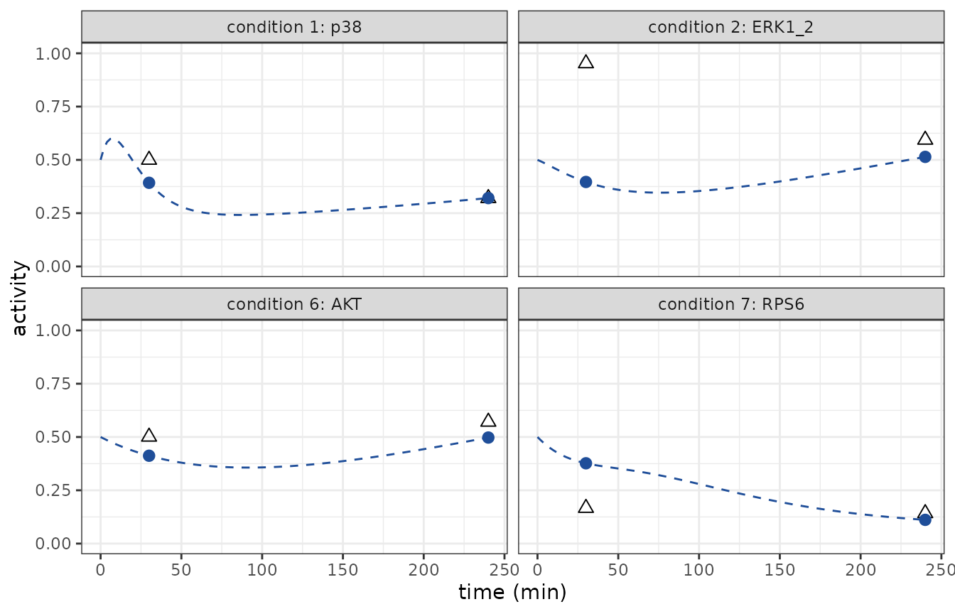
Model simulation (line) against the measured normalised activity (points) for four representative condition / phosphoprotein pairs, in the style of the Figure 3b upper panels.
Validation checks
This model has no drug, no dose and no plasma concentration, so a PKNCA non-compartmental analysis is not the right instrument. The checks below are the mechanistic-model equivalents: exact structural identities, an independent closed-form steady state, and the paper’s own qualitative claims.
1. Nodes with tau = 0 are frozen at basal, in every
condition
tau_IGF1_R, tau_TNFR and
tau_IKKa are all exactly zero in the fitted parameter set,
so the whole right-hand side of those three ODEs vanishes and the states
cannot leave their initial value.
2. The system does not respond to IGF-1 or TNF-alpha
Traynard 2017 draws a biological conclusion from those three null lifetimes: “IGF1-R, TNFR, and IKK are associated with null tau parameters, which means that they become independent from their regulator activities. The system therefore does not depend on the inputs IGF-1 and TNF alpha.” If the packaged model is right, turning those two ligands on must change nothing, anywhere, at any time – exactly, not approximately.
states <- rxode2::rxState(mod)
control <- dplyr::mutate(
  design[1, ],
  STIM_EGF_NORM = 0.5, STIM_IGF1_NORM = 0.5, STIM_IL6_NORM = 0.5,
  STIM_TNFA_NORM = 0.5, STIM_DHT_NORM = 0.5,
  PI3K_INHIBITED = 0, MEK_INHIBITED = 0, MTOR_INHIBITED = 0, P38_INHIBITED = 0, IKK_INHIBITED = 0
)
tgrid <- as.data.frame(rxode2::et(seq(0, 240, by = 5)))
solve_one <- function(p) {
  p$id <- 1L
  rxode2::rxSolve(mod, events = cbind(id = 1L, tgrid), params = p, returnType = "data.frame")
}

base_traj <- as.matrix(solve_one(control)[, states])
dev_igf1 <- max(abs(as.matrix(solve_one(dplyr::mutate(control, STIM_IGF1_NORM = 1))[, states]) - base_traj))
dev_tnfa <- max(abs(as.matrix(solve_one(dplyr::mutate(control, STIM_TNFA_NORM = 1))[, states]) - base_traj))

c(IGF1 = dev_igf1, TNFa = dev_tnfa)
#> IGF1 TNFa
#>    0    0
stopifnot(dev_igf1 == 0, dev_tnfa == 0)
3. A fully inhibited node is pinned at the basal value
inh_map <- c(PI3K = "PI3K_INHIBITED", MEK = "MEK_INHIBITED", mTOR = "MTOR_INHIBITED", p38 = "P38_INHIBITED", IKKa = "IKK_INHIBITED")
stimulated <- dplyr::mutate(control, STIM_EGF_NORM = 1, STIM_DHT_NORM = 1, STIM_IL6_NORM = 1)

dev_inh <- vapply(names(inh_map), function(nm) {
  p <- stimulated
  p[[inh_map[[nm]]]] <- 1
  max(abs(solve_one(p)[[nm]] - 0.5))
}, numeric(1))

dev_inh
#> PI3K  MEK mTOR  p38 IKKa
#>    0    0    0    0    0
stopifnot(all(dev_inh == 0))
4. The ODE steady state matches an independent closed-form fixed point
The trained network is a directed acyclic graph apart from a single
AR -> PI3K -> AKT -> AR feedback loop. Its steady
state can therefore be computed without any ODE solver: substitute
forward through the cascade, and resolve the one loop by fixed-point
iteration. The transfer function used below is written out again from
the CNORode2017 C source rather than reused from the model
object, so this is an independent check of the packaged ODEs, not a
restatement of them.
fg <- function(x, k, n = 3) 1 - (1 - x)^n / ((1 - x)^n + k^n) * (1 + k^n)

closed_form_ss <- function(EGF, IGF1, IL6, TNFa, DHT) {
  EGFR <- fg(EGF, 0.550337329553758)
  IGF1_R <- 0.5 # tau = 0
  IL6R <- fg(IL6, 0.78134194522735)
  TNFR <- 0.5 # tau = 0
  # The one feedback loop AR -> PI3K -> AKT -> AR, resolved by fixed-point
  # iteration; the map is a contraction here so it converges in a few steps.
  AR <- AKT <- PI3K <- 0.5
  repeat {
    prev <- c(AR, PI3K, AKT)
    AR <- 1 - (1 - fg(AKT, 0.000835340126624366)) * (1 - fg(DHT, 0.590287658825809))
    PI3K <- 1 - (1 - fg(AR, 1)) * (1 - fg(EGFR, 1)) * (1 - fg(IGF1_R, 1))
    AKT <- fg(PI3K, 0.352193224711085)
    if (max(abs(c(AR, PI3K, AKT) - prev)) < 1e-15) break
  }
  mTOR <- fg(AKT, 1)
  Jak <- fg(IL6R, 1)
  RAS <- 1 - (1 - fg(Jak, 0.674347577514922)) * (1 - fg(EGFR, 0.25869659979145))
  Rac <- fg(RAS, 0.284328823821596)
  p38 <- fg(Rac, 1)
  c(
    EGFR = EGFR, IGF1_R = IGF1_R, IL6R = IL6R, TNFR = TNFR, AR = AR, PI3K = PI3K,
    AKT = AKT, mTOR = mTOR, RPS6 = fg(mTOR, 0.303674761072917),
    GSK3a = fg(AKT, 0.558225196843653), Jak = Jak, Stat3 = fg(Jak, 0.28320076784032),
    RAS = RAS, MEK = fg(RAS, 0.490290337695327),
    ERK1_2 = fg(fg(RAS, 0.490290337695327), 0.462172528684214), Rac = Rac, p38 = p38,
    HSP27 = fg(p38, 0.993983089528085),
    JNK = 1 - (1 - fg(TNFR, 0.361795499785572)) * (1 - fg(Rac, 0.0000673323536405412)),
    IKKa = 0.5
  )
}

scenarios <- tibble::tribble(
  ~label, ~EGF, ~IGF1, ~IL6, ~TNFa, ~DHT,
  "control", 0.5, 0.5, 0.5, 0.5, 0.5,
  "EGF", 1.0, 0.5, 0.5, 0.5, 0.5,
  "DHT", 0.5, 0.5, 0.5, 0.5, 1.0,
  "EGF + IL6 + DHT", 1.0, 0.5, 1.0, 0.5, 1.0
)

ss_long_grid <- as.data.frame(rxode2::et(c(0, 2e6)))
ss_dev <- vapply(seq_len(nrow(scenarios)), function(i) {
  p <- dplyr::mutate(
    control,
    STIM_EGF_NORM = scenarios$EGF[i], STIM_IGF1_NORM = scenarios$IGF1[i],
    STIM_IL6_NORM = scenarios$IL6[i], STIM_TNFA_NORM = scenarios$TNFa[i],
    STIM_DHT_NORM = scenarios$DHT[i]
  )
  p$id <- 1L
  sv <- rxode2::rxSolve(mod, events = cbind(id = 1L, ss_long_grid), params = p, returnType = "data.frame")
  ana <- closed_form_ss(scenarios$EGF[i], scenarios$IGF1[i], scenarios$IL6[i], scenarios$TNFa[i], scenarios$DHT[i])
  max(abs(unlist(sv[nrow(sv), states]) - ana[states]))
}, numeric(1))

knitr::kable(
  dplyr::mutate(scenarios["label"], `max abs deviation` = signif(ss_dev, 3)),
  caption = "ODE solution at t = 2e6 min versus the closed-form fixed point."
)| label | max abs deviation |
|---|---|
| control | 0 |
| EGF | 0 |
| DHT | 0 |
| EGF + IL6 + DHT | 0 |
5. The EGF arm dominates, and the IL-6 arm barely moves
Traynard 2017: “IL6-R is associated with a very small value for tau(IL6-R), suggesting that the dynamics of the system will predominantly depend on pathways activated by EGF.”
arm_shift <- function(stim) {
  p <- control
  p[[stim]] <- 1
  max(abs(as.matrix(solve_one(p)[, states]) - base_traj))
}
shifts <- vapply(
  c(EGF = "STIM_EGF_NORM", IL6 = "STIM_IL6_NORM", DHT = "STIM_DHT_NORM"),
  arm_shift, numeric(1)
)
round(shifts, 4)
#>    EGF    IL6    DHT
#> 0.5000 0.0223 0.4557

# Deterministic solves, so these are exact numbers, not a sampled cohort. The
# EGF arm moves the network more than twenty times as far as the IL-6 arm, and
# the IL-6 arm barely leaves basal at all.
stopifnot(
  shifts[["EGF"]] > 10 * shifts[["IL6"]],
  shifts[["DHT"]] > 10 * shifts[["IL6"]],
  shifts[["IL6"]] < 0.05
)
The EGF arm shifts the network by up to 0.50 activity units and the androgen arm by 0.46, against 0.022 for IL-6 – the IL-6 receptor’s lifetime parameter is small enough (3.1e-04 per min) that its arm has hardly begun to move by 240 min.
6. Androgen and PI3K inhibition at the node level
Table 1 of Traynard 2017 compares experimental survival proportions against MaBoSS survival probabilities. Survival is not a state of the logic-based ODE model (see Assumptions below), but the node-level behaviour that drives the paper’s conclusion – DHT raises PI3K/AKT signaling, and PI3K inhibition abrogates it – is reproducible here.
arm <- function(lab, dht, pi3ki) {
  p <- dplyr::mutate(control, STIM_DHT_NORM = dht, PI3K_INHIBITED = pi3ki)
  p$id <- 1L
  sv <- rxode2::rxSolve(mod, events = cbind(id = 1L, tgrid), params = p, returnType = "data.frame")
  tibble::tibble(
    Condition = lab,
    AR = sv$AR[nrow(sv)], PI3K = sv$PI3K[nrow(sv)], AKT = sv$AKT[nrow(sv)],
    mTOR = sv$mTOR[nrow(sv)], RPS6 = sv$RPS6[nrow(sv)]
  )
}
t1 <- dplyr::bind_rows(
  arm("control (DHT absent)", 0.5, 0),
  arm("DHT = 1", 1.0, 0),
  arm("PI3K inhibited", 0.5, 1),
  arm("DHT = 1 + PI3K inhibited", 1.0, 1)
)
knitr::kable(dplyr::mutate(t1, dplyr::across(-Condition, ~ round(.x, 3))),
  caption = "Node activity at 240 min in the Table 1 androgen / PI3K-inhibitor conditions."
)| Condition | AR | PI3K | AKT | mTOR | RPS6 |
|---|---|---|---|---|---|
| control (DHT absent) | 0.544 | 0.695 | 0.492 | 0.708 | 0.398 |
| DHT = 1 | 1.000 | 0.698 | 0.497 | 0.714 | 0.408 |
| PI3K inhibited | 0.544 | 0.500 | 0.236 | 0.398 | 0.111 |
| DHT = 1 + PI3K inhibited | 1.000 | 0.500 | 0.236 | 0.398 | 0.111 |
# DHT must raise AR and the PI3K axis; PI3K inhibition must pin the axis at basal
# and block the DHT effect downstream of PI3K.
stopifnot(
  t1$AR[2] > t1$AR[1],
  t1$PI3K[2] > t1$PI3K[1],
  t1$AKT[2] > t1$AKT[1],
  t1$PI3K[3] == 0.5, t1$PI3K[4] == 0.5,
  t1$AKT[4] == t1$AKT[3]
)
DHT raises AR and propagates through PI3K, AKT, mTOR and RPS6; inhibiting PI3K pins the axis at basal and the DHT signal cannot reach AKT at all, which is the node-level counterpart of the survival result the paper reports (survival 0.87 with DHT, 0.33 with PI3K inhibition, 0.63 with both).
Assumptions and deviations
-
The MaBoSS Boolean model is not packaged. Traynard
2017 builds two models. The one packaged here is the logic-based ODE
model trained with CellNOptR. The second is a continuous-time Markov
process over Boolean states, simulated with MaBoSS, over the full
uncompressed network including
Survival,Cell_cycle,MYC,Caspase8,Caspase9,p53,NFkBandbeta_catenin. That model is not an ODE system – it is a stochastic jump process whose master equation runs over2^nBoolean states – so it cannot be expressed in rxode2, and the eight extra nodes it carries were removed from the ODE model by CellNOptR’s compression step and have no fitted parameters. The survival probabilities in Table 1, the node-inhibition scan in Figure 5 and the epistasis network in Figure 6 are all MaBoSS outputs and are therefore out of scope for this file. The MaBoSS model definition is in the supplement astrainedmodel.bnd/trainedmodel.cfgfor anyone who wants it. -
The trained model has 25 edges; the published prior
knowledge network file has 26 candidate edges among the surviving
nodes.
PriorKnowledgeNetwork.sifcontains a final lineTNFa -> PI3Kthat is absent from the fitted parameter filelogicODEparameters_edges.txt, absent from the trained MaBoSS model (trainedmodel.bndgives PI3K the ruleAR | EGFR | IGF1_R), and not drawn in Figure 3a. The.siffile has classic-Mac CR line endings and no terminating newline on that last line, which is the likely reason it was not read at training time. Two independent published artifacts agree on the 25-edge trained model, so that is what is packaged; the discrepancy is recorded here rather than silently resolved. -
Parameters are on the natural scale, not
log-transformed.
tauandkare bounded on[0, 1]by the fitting script and several estimates sit exactly on a bound (tau = 0for three nodes,k = 1for six edges), so a log parameterization is both undefined and structurally wrong here. - No IIV and no residual error. Traynard 2017 reports a single deterministic fit obtained by minimizing a residual sum of squares plus a steady-state penalty. No parameter standard errors, confidence intervals, between-subject variances or residual-error terms are reported anywhere in the paper or its supplement; uncertainty is reported only as a bootstrap performance distribution in Figure 3d. Nothing was invented to fill those gaps.
-
Ligand and inhibitor concentrations are not recoverable from
this paper. The applied concentrations live in Lescarbeau 2014,
the upstream data paper. The
STIM_*covariates are therefore expressed on the model’s own normalized activity scale (0.5 = absent, 1 = applied) and the*_INHIBITEDcovariates are binary flags, which is exactly the resolution the trained model uses. -
Inhibition pins a node at basal rather than driving it to
zero. This is the
CNORode2017convention (src/rhsODE.cmultiplies the whole derivative by1 - inhibitor), and it is coherent with the normalization in which 0.5 is the unperturbed basal state: the inhibitor prevents the node from responding, it does not abolish baseline activity. The covariates accept values on[0, 1]so a partial inhibition can be simulated, although the Lescarbeau 2014 design used 0/1 only. -
The GSK3 antibody measures an inhibitory site.
Traynard 2017 inverted the sign of the edges to and from GSK3 to account
for this before fitting; the
GSK3astate and its fittedk_AKT_GSK3atherefore already carry that inversion, and no further sign handling is applied here. -
The Hill exponent is a single shared parameter.
CNORode carries one
nper edge, but the fitting script fixed every one of them at the default of 3 (opt_n = FALSE), so a singlenhillparameter is an exact representation of the published model. -
Source is the supplementary repository, not the article
PDF. The article prints the structural ODE form and two of the
25 edge strengths (
k(Rac -> JNK)andk(AKT -> AR), both of which match the supplement exactly); all remaining parameter values come from the GitHub repository the article’s Supplementary Materials section designates. The relevant files were available alongside the article PDF when this model was built. -
Transfer-function and right-hand-side semantics were read
from source. The article does not write out
FG_transfer_functionor the inhibitor factor; those were read from the C sources ofCNORode2017, the package the supplement’s own fitting script installs and calls. The Figure 3c answer key (Pearson correlation 0.66 and MSE 0.017) confirms the reading.
Session info
sessionInfo()
#> R version 4.6.1 (2026-06-24)
#> Platform: x86_64-pc-linux-gnu
#> Running under: Ubuntu 24.04.5 LTS
#>
#> Matrix products: default
#> BLAS:   /usr/lib/x86_64-linux-gnu/openblas-pthread/libblas.so.3
#> LAPACK: /usr/lib/x86_64-linux-gnu/openblas-pthread/libopenblasp-r0.3.26.so;  LAPACK version 3.12.0
#>
#> locale:
#>  [1] LC_CTYPE=C.UTF-8       LC_NUMERIC=C           LC_TIME=C.UTF-8
#>  [4] LC_COLLATE=C.UTF-8     LC_MONETARY=C.UTF-8    LC_MESSAGES=C.UTF-8
#>  [7] LC_PAPER=C.UTF-8       LC_NAME=C              LC_ADDRESS=C
#> [10] LC_TELEPHONE=C         LC_MEASUREMENT=C.UTF-8 LC_IDENTIFICATION=C
#>
#> time zone: UTC
#> tzcode source: system (glibc)
#>
#> attached base packages:
#> [1] stats     graphics  grDevices utils     datasets  methods   base
#>
#> other attached packages:
#> [1] ggplot2_4.0.3         tidyr_1.3.2           dplyr_1.2.1
#> [4] rxode2_5.1.8          nlmixr2lib_0.3.2.9000
#>
#> loaded via a namespace (and not attached):
#>  [1] gtable_0.3.6        xfun_0.61           bslib_0.12.0
#>  [4] rxode2lincmt_0.1.0  lattice_0.22-9      vctrs_0.7.3
#>  [7] tools_4.6.1         generics_0.1.4      parallel_4.6.1
#> [10] tibble_3.3.1        symengine_0.2.14    pkgconfig_2.0.3
#> [13] Matrix_1.7-5        data.table_1.18.6.1 checkmate_2.3.4
#> [16] RColorBrewer_1.1-3  S7_0.2.2            desc_1.4.3
#> [19] lifecycle_1.0.5     compiler_4.6.1      farver_2.1.2
#> [22] textshaping_1.0.5   fontawesome_0.5.3   htmltools_0.5.9
#> [25] sys_3.4.3           sass_0.4.10         yaml_2.3.12
#> [28] pillar_1.11.1       pkgdown_2.2.1       crayon_1.5.3
#> [31] jquerylib_0.1.4     whisker_0.4.1       openssl_2.4.2
#> [34] cachem_1.1.0        nlme_3.1-169        tidyselect_1.2.1
#> [37] digest_0.6.39       lotri_1.0.5         purrr_1.2.2
#> [40] labeling_0.4.3      splines_4.6.1       rxode2ll_2.0.18
#> [43] fastmap_1.2.0       grid_4.6.1          cli_3.6.6
#> [46] dparser_1.3.1-14    magrittr_2.0.5      withr_3.0.3
#> [49] scales_1.4.0        backports_1.5.1     rmarkdown_2.32
#> [52] otel_0.2.0          askpass_1.2.1       ragg_1.5.2
#> [55] memoise_2.0.1       evaluate_1.0.5      knitr_1.52
#> [58] rex_1.2.2           mgcv_1.9-4          PreciseSums_0.7
#> [61] rlang_1.3.0         downlit_0.4.5       Rcpp_1.1.2
#> [64] glue_1.8.1          xml2_1.6.0          jsonlite_2.0.0
#> [67] R6_2.6.1            systemfonts_1.3.2   fs_2.1.0