Elagolix bone QSP (Stodtmann 2021)
Source:vignettes/articles/Stodtmann_2021_elagolix.Rmd
Stodtmann_2021_elagolix.RmdModel and source
- Citation: Stodtmann S, Nader A, Polepally AR, Suleiman AA, Winzenborg I, Noertersheuser P, Ng J, Mostafa NM, Shebley M. Validation of a quantitative systems pharmacology model of calcium homeostasis using elagolix Phase 3 clinical trial data in women with endometriosis. Clin Transl Sci. 2021;14:1611-1619. doi:10.1111/cts.13040. The dose-E2 model (equation 3, Table 2) is from that paper. The QSP model was applied there without modification from Riggs MM, Bennetts M, van der Graaf PH, Martin SW. Integrated pharmacometrics and systems pharmacology model-based analyses to guide GnRH receptor modulator development for management of endometriosis. CPT Pharmacometrics Syst Pharmacol. 2012;1:e11. doi:10.1038/psp.2012.10, which supplies the estrogen effects (equations 2-5), the E2 scaling function (equation 6) and the lumbar spine BMD equation (equation 7). Riggs 2012 in turn fixes every other system value to Peterson MC, Riggs MM. Bone. 2010;46(1):49-63. doi:10.1016/j.bone.2009.08.053; those backbone equations and values are transcribed from the authors’ open-source release of the same model, https://github.com/metrumresearchgroup/OpenBoneMin, file inst/OpenBoneMin.cpp at commit b3d59bfc (2026-01-26), whose estrogen block carries the Riggs 2012 extension. Differences between the printed Riggs 2012 values and the code are listed in the validation vignette.
- Description: QSP. Elagolix dose-estradiol model coupled to the Peterson-Riggs calcium-homeostasis and bone-remodelling systems pharmacology model with the Riggs 2012 estrogen extension, predicting lumbar spine bone mineral density (BMD) and the bone-turnover markers serum CTX (resorption) and P1NP (formation) in premenopausal women with endometriosis. An empirical shifted/scaled-logit function of the total daily elagolix dose gives the average serum estradiol (E2) level; E2 relative to its untreated level is mapped to a fractional estrogen effect through the Riggs 2012 sigmoid scaling function, which acts on latent and active TGF-beta, responding osteoblasts, osteoblast apoptosis and the renal tubular calcium-reabsorption maximum of the 29-state calcium / PTH / calcitriol / phosphate / RANK-RANKL-OPG / osteoblast-osteoclast / RUNX2-CREB-BCL2 backbone. Lumbar spine BMD follows an indirect-response equation driven by relative osteoblast (formation) and osteoclast (resorption) activity. Deterministic typical-value model: no IIV and no residual error.
- Article: https://doi.org/10.1111/cts.13040
- QSP model applied by the article (Riggs 2012): https://doi.org/10.1038/psp.2012.10
- Structural source for the calcium / bone backbone: https://github.com/metrumresearchgroup/OpenBoneMin
Stodtmann et al. link elagolix, an oral gonadotropin-releasing hormone receptor antagonist, to lumbar spine bone mineral density (BMD) in two steps:
- an empirical dose-E2 model – a shifted/scaled logit of the total daily elagolix dose that returns the average serum estradiol (E2) level (equation 3, Table 2), estimated in the paper; and
- the calcium-homeostasis / bone-remodelling QSP model of Peterson and Riggs with the estrogen extension of Riggs et al. 2012, applied “without any modification”, which turns E2 into lumbar spine BMD, serum CTX (resorption) and P1NP (formation).
The packaged model is the coupled system. It is deterministic (no
IIV, no residual error) and has no elagolix pharmacokinetics: E2 is a
steady-state function of the daily dose, supplied as the time-varying
covariate DOSE_ELAGOLIX_MGD. Non-compartmental analysis is
therefore not an appropriate check. The vignette instead reproduces the
paper’s Figure 1 dose-E2 curve, its Table 3 predicted BMD changes,
Figures 2-4, and the Riggs 2012 benchmark on which the bone model was
built.
mod <- readModelDb("Stodtmann_2021_elagolix")
ui <- rxode2::rxode2(mod)
length(ui$state)
#> [1] 30
Population
The dose-E2 model was fit to average E2 levels from six elagolix studies in premenopausal women (Stodtmann 2021 Table 1): a phase 1 study in healthy volunteers (100/150/200 mg once daily, 100/200/300 mg twice daily and 600 mg once daily for three menstrual cycles, E2 sampled three times a week), a phase 2b study in women with heavy menstrual bleeding from uterine fibroids, and four phase 3 studies in women with moderate to severe endometriosis-associated pain (Elaris EM-I and EM-II, 150 mg once daily or 200 mg twice daily for 6 months, and their 6-month extensions EM-III and EM-IV with 6 months of post-treatment follow-up). Weighted nonlinear least squares was used, weighting each regimen by its cohort size and up-weighting the intensively sampled phase 1 study. The paper does not tabulate demographics; they are published with each trial.
The QSP model was not refit: the phase 3 BMD, CTX and P1NP data served only as external validation.
str(mod()$population)
#> List of 9
#>  $ species       : chr "human"
#>  $ n_subjects    : logi NA
#>  $ n_studies     : num 6
#>  $ age_range     : chr "premenopausal adult women (individual demographics not reported in this paper)"
#>  $ sex_female_pct: num 100
#>  $ disease_state : chr "Premenopausal women: healthy volunteers (phase 1), women with heavy menstrual bleeding associated with uterine "| __truncated__
#>  $ dose_range    : chr "Elagolix 100/150/200 mg once daily, 100/200/300 mg twice daily and 600 mg once daily (total daily dose 0-600 mg"| __truncated__
#>  $ regions       : chr "multinational (phase 3 Elaris EM program)"
#>  $ notes         : chr "The dose-E2 model was fit by weighted nonlinear least squares to mean E2 levels from all six studies of Table 1"| __truncated__
Source trace
Dose-E2 model (the part estimated in Stodtmann 2021)
| Equation / parameter | Value | Source location |
|---|---|---|
e2 = E2min + (E2max - E2min) / (1 + exp(slope * DailyDose)) |
– | Stodtmann 2021 equation 3 |
e2slope |
0.00894 per mg/day | Table 2 ‘Slope’ |
lE2max |
5.20 (E2max = 181.3 pg/mL) | Table 2 ‘Log(E2max)’ |
lE2min |
2.14 (E2min = 8.50 pg/mL) | Table 2 ‘Log(E2min)’ |
| Untreated E2 = (E2max + E2min) / 2 = 94.9 pg/mL | – | Table 2 footnote |
Estrogen coupling (Riggs 2012, applied unchanged)
| Equation / parameter | Value | Source location |
|---|---|---|
E2frac = e2 / E2ref |
E2ref = 100 pg/mL |
Riggs 2012 p 2, “assuming a typical baseline E2 of ~100 pg/ml” |
E = E2frac^2.1 / (E2frac^2.1 + 0.15^2.1) |
E2gam = 2.1, E2frac50 = 0.15 |
Riggs 2012 equation 6 |
Latent TGF-beta production * (1/E)^tgfbGAM
|
tgfbGAM = 0.075 |
Riggs 2012 equation 2 and p 4 |
Latent-to-active TGF-beta conversion
* E^tgfbactGAM
|
tgfbactGAM = 0.045 |
Riggs 2012 equations 2-3 and p 4 |
Responding-osteoblast production * (1/E)^robGAM
|
robGAM = 0.16 |
Riggs 2012 equation 4 and p 4 |
Active-osteoblast apoptosis * (1/E)^E2scalePicB1
|
E2scalePicB1 = 0.000012 |
Riggs 2012 equation 5 and p 4 |
| Tubular Ca-reabsorption maximum, linear in E |
maxTmESTkid = 0.923737 |
Riggs 2012 p 4 (“~8% decline … with a 90% estrogen reduction”); value from OpenBoneMin line 214 |
d(BMD)/dt = kin * (OB/OB0)^gamOB - kout * (OC/OC0)^gamOCls * BMD |
– | Riggs 2012 equation 7; OpenBoneMin line 679 |
koutBMDls |
0.000397 /h (0.00953 /day) | Riggs 2012 p 4 (see “Errata”); OpenBoneMin line 170 |
gamOCls |
0.14 | Riggs 2012 p 4 (see “Errata”); OpenBoneMin line 174 |
gamOB |
0.0739 | Riggs 2012 p 4 |
Calcium / bone backbone (Peterson and Riggs 2010)
Riggs 2012 states that, apart from the parameters above, “all other
model parameters were considered as system values and fixed at the
previously reported values” of Peterson and Riggs 2010. That backbone –
29 states covering plasma calcium, phosphate, PTH and the parathyroid
gland, calcitriol and 1-alpha-hydroxylase, gut absorption, exchangeable
and non-exchangeable bone calcium, the RANK / RANKL / OPG axis,
osteoblast and osteoclast populations, latent and active TGF-beta, and
the RUNX2 / CREB / BCL-2 cascade – is transcribed from
inst/OpenBoneMin.cpp in the authors’ open-source release
(commit b3d59bfc). Every backbone value in the model file carries an
obm:NNN comment giving its line in that file. The
transcription is shared with the Riggs_2012_ckd_mbd_qsp
model in this package. When this model was added, the coupled model was
run side by side with OpenBoneMin.cpp itself (compiled with
mrgsolve) at the code’s own estrogen exponents and an identical constant
estrogen fraction: lumbar spine BMD at 6, 12, 18 and 24 months agreed to
four significant figures for both elagolix regimens, as did CTX and P1NP
at 12 months.
State-name mapping
| This model | OpenBoneMin.cpp |
Meaning |
|---|---|---|
PTH |
PTH |
plasma parathyroid hormone (pmol) |
PTpool |
S |
parathyroid gland PTH-production capacity |
PThypertrophy |
PTmax |
parathyroid gland hypertrophy factor |
calcitriol |
B |
plasma calcitriol (pmol) |
alphaOHase |
AOH |
renal 1-alpha-hydroxylase |
plasmaCa |
P |
plasma calcium (mmol) |
ECCPhos |
ECCPhos |
extracellular phosphate (mmol) |
PhosGut |
PhosGut |
dietary phosphate in gut (mmol) |
IntraPO |
IntraPO |
intracellular phosphate (mmol) |
gutCa |
T |
dietary calcium in gut (mmol) |
gutCaAbsorp |
R |
calcitriol-dependent gut absorption capacity |
HAp |
HAp |
hydroxyapatite deposition capacity |
boneCaExch |
Q |
immediately exchangeable bone calcium (mmol) |
boneCaNonExch |
Qbone |
non-exchangeable bone calcium (mmol) |
OBfast, OBslow
|
OBfast, OBslow
|
osteoblast pools |
OC |
OC |
active osteoclasts |
ROB |
ROB1 |
responding osteoblasts |
TGFB, TGFBact
|
TGFB, TGFBact
|
latent and active TGF-beta |
RANKL |
L |
free RANK ligand |
RANK |
RNK |
free RANK |
RANK_RANKL |
M |
RANK-RANKL complex |
OPG |
O |
free osteoprotegerin |
OPG_RANKL |
N |
OPG-RANKL complex |
RX2, CREB, BCL2
|
RX2, CREB, BCL2
|
intracellular cascade |
BMDls |
BMDls |
lumbar spine bone mineral density (ratio to baseline) |
urineCa |
UCA |
cumulative urinary calcium (mmol) |
EST (algebraic) |
EST |
estrogen fraction E of Riggs 2012 |
Outputs
| Output | Definition | Paper quantity |
|---|---|---|
e2 |
dose-E2 model prediction (pg/mL) | Figure 1 |
EST |
estrogen fraction E (unitless) | Riggs 2012 equation 6 |
BMDlspct |
(BMDls - 1) * 100 |
lumbar spine BMD, % change from baseline |
CTXchgpct |
100 * (OC / OC0 - 1) |
CTX, % change from baseline |
P1NPchgpct |
100 * (OB / OB0 - 1) |
P1NP, % change from baseline |
Simulation helpers
Time is in hours (the OpenBoneMin convention); one month is 8766 / 12
h. A treatment sequence is a table of switch times and daily doses,
expanded onto a weekly observation grid. Observation rows are placed on
the BMDls state; every algebraic output is returned
alongside it.
hours_per_month <- 8766 / 12

simulate_sequence <- function(start_month, daily_dose, end_month = 36, by = 0.25) {
  month <- seq(0, end_month, by = by)
  events <- data.frame(
    id = 1,
    time = month * hours_per_month,
    evid = 0,
    cmt = "BMDls",
    DOSE_ELAGOLIX_MGD = daily_dose[findInterval(month, start_month)]
  )
  sim <- rxode2::rxSolve(
    ui,
    events,
    returnType = "data.frame",
    atol = 1e-10,
    rtol = 1e-8,
    maxsteps = 1e6
  )
  sim$month <- sim$time / hours_per_month
  sim
}

value_at <- function(sim, month, column = "BMDlspct") {
  sim[[column]][abs(sim$month - month) < 1e-6]
}
Check 1: the dose-E2 model (Figure 1)
dose_grid <- seq(0, 600, by = 5)
e2_grid <- rxode2::rxSolve(
  ui,
  data.frame(id = seq_along(dose_grid), time = 0, evid = 0, cmt = "BMDls",
             DOSE_ELAGOLIX_MGD = dose_grid),
  returnType = "data.frame"
)
e2_curve <- data.frame(dose = dose_grid, e2 = e2_grid$e2)

ggplot(e2_curve, aes(dose, e2)) +
  geom_line(linewidth = 1) +
  scale_x_continuous(breaks = c(0, 100, 150, 200, 400, 600)) +
  labs(x = "Daily dose (mg)", y = "Estradiol (pg/mL)",
       caption = "Replicates the fitted line of Figure 1 of Stodtmann 2021.")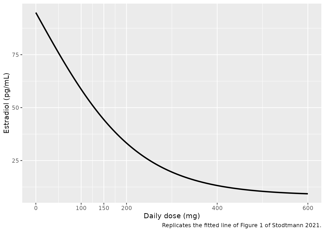
The curve starts at the untreated level of the Table 2 footnote and falls to the ~10 pg/mL the paper reports at 600 mg/day.
e2_at <- function(d) e2_curve$e2[e2_curve$dose == d]
e2_checks <- data.frame(
  daily_dose = c(0, 150, 400, 600),
  e2 = c(e2_at(0), e2_at(150), e2_at(400), e2_at(600))
)
knitr::kable(e2_checks, digits = 1)| daily_dose | e2 |
|---|---|
| 0 | 94.9 |
| 150 | 44.3 |
| 400 | 13.2 |
| 600 | 9.3 |
Check 2: the untreated system
At DOSE_ELAGOLIX_MGD = 0 the dose-E2 model gives 94.9
pg/mL, an E2 fraction of 0.949 against the Riggs 2012 reference of 100
pg/mL, and an estrogen fraction E of 0.980 rather than exactly 1. Both
are properties of the published equations (equation 6 itself gives E =
0.982 at an E2 fraction of 1). The untreated system therefore drifts
very slightly from the bone model’s premenopausal steady state:
untreated <- simulate_sequence(0, 0, end_month = 24)
drift <- data.frame(
  month = c(6, 12, 18, 24),
  BMD = sapply(c(6, 12, 18, 24), value_at, sim = untreated),
  CTX = sapply(c(6, 12, 18, 24), value_at, sim = untreated, column = "CTXchgpct"),
  P1NP = sapply(c(6, 12, 18, 24), value_at, sim = untreated, column = "P1NPchgpct")
)
drift |>
  dplyr::rename("Month" = month, "BMD change (%)" = BMD,
                "CTX change (%)" = CTX, "P1NP change (%)" = P1NP) |>
knitr::kable(digits = 2)| Month | BMD change (%) | CTX change (%) | P1NP change (%) |
|---|---|---|---|
| 6 | -0.13 | 1.80 | 0.81 |
| 12 | -0.19 | 1.98 | 0.98 |
| 18 | -0.19 | 1.77 | 0.85 |
| 24 | -0.17 | 1.52 | 0.68 |
A drift of under 0.2% in BMD over two years is well inside the paper’s validation RMSE (0.68-0.78% for BMD, Table S2) and is invisible in the placebo segments of Figure 3.
Check 3: the Riggs 2012 benchmark
Riggs 2012 states that “continuous suppression of estrogen by 80% for 6 months was expected to cause a 2% BMD loss” and marks a “Reference (-2.2%)” line on its Figure 4. The daily elagolix dose that gives E2 = 20 pg/mL (80% suppression against 100 pg/mL) is found by inverting equation 3.
dose_for_e2 <- function(e2_target) {
  log((exp(5.20) - exp(2.14)) / (e2_target - exp(2.14)) - 1) / 0.00894
}
riggs80 <- simulate_sequence(0, dose_for_e2(20), end_month = 6)
riggs60 <- simulate_sequence(0, dose_for_e2(40), end_month = 6)
riggs_tab <- data.frame(
  suppression = c("80% (E2 20 pg/mL)", "60% (E2 40 pg/mL)"),
  daily_dose = c(dose_for_e2(20), dose_for_e2(40)),
  bmd6 = c(value_at(riggs80, 6), value_at(riggs60, 6)),
  riggs = c("~ -2% (Figure 4 reference -2.2%)", "~ -1%")
)
riggs_tab |>
  dplyr::rename("E2 suppression" = suppression, "Daily dose (mg)" = daily_dose,
                "Simulated 6-month BMD change (%)" = bmd6,
                "Riggs 2012" = riggs) |>
knitr::kable(digits = 2)| E2 suppression | Daily dose (mg) | Simulated 6-month BMD change (%) | Riggs 2012 |
|---|---|---|---|
| 80% (E2 20 pg/mL) | 295.38 | -2.26 | ~ -2% (Figure 4 reference -2.2%) |
| 60% (E2 40 pg/mL) | 167.86 | -0.74 | ~ -1% |
Check 4: Table 3, continuous dosing for 24 months
cont150 <- simulate_sequence(0, 150, end_month = 24)
cont400 <- simulate_sequence(0, 400, end_month = 24)
months <- c(6, 12, 18, 24)
table3 <- data.frame(
  regimen = rep(c("150 mg q.d.", "200 mg b.i.d."), each = 4),
  month = rep(months, 2),
  published = c(-0.61, -0.91, -0.96, -0.91, -3.47, -4.95, -5.15, -4.97),
  simulated = c(sapply(months, value_at, sim = cont150),
                sapply(months, value_at, sim = cont400))
)
table3$difference <- table3$simulated - table3$published
table3 |>
  dplyr::rename("Regimen" = regimen, "Month" = month,
                "Published QSP (%)" = published, "Simulated (%)" = simulated,
                "Difference (pp)" = difference) |>
knitr::kable(digits = 2)| Regimen | Month | Published QSP (%) | Simulated (%) | Difference (pp) |
|---|---|---|---|---|
| 150 mg q.d. | 6 | -0.61 | -0.61 | 0.00 |
| 150 mg q.d. | 12 | -0.91 | -0.88 | 0.03 |
| 150 mg q.d. | 18 | -0.96 | -0.89 | 0.07 |
| 150 mg q.d. | 24 | -0.91 | -0.81 | 0.10 |
| 200 mg b.i.d. | 6 | -3.47 | -3.53 | -0.06 |
| 200 mg b.i.d. | 12 | -4.95 | -4.94 | 0.01 |
| 200 mg b.i.d. | 18 | -5.15 | -5.00 | 0.15 |
| 200 mg b.i.d. | 24 | -4.97 | -4.72 | 0.25 |
The 6- and 12-month predictions – the horizon the phase 3 data cover and the one the paper validated – agree to within 0.06 percentage points. The 18- and 24-month extrapolations agree to within 0.25 percentage points; the packaged model reaches its nadir about two months earlier than the published curve (see “Assumptions and deviations”).
on_trial <- table3$month <= 12
nadir_month <- cont400$month[which.min(cont400$BMDlspct)]
nadir_month
#> [1] 15.25
stopifnot(
  max(abs(table3$difference[on_trial])) < 0.1,
  max(abs(table3$difference)) < 0.3,
  nadir_month > 13, nadir_month < 17
)
Three choices the paper does not state explicitly were settled against this table (see “Assumptions and deviations”). Each alternative is a parameter override of the packaged model; the root mean square error across the eight Table 3 cells is lowest for the packaged choices.
table3_rmse <- function(params = NULL) {
  pred <- unlist(lapply(c(150, 400), function(d) {
    ev <- data.frame(id = 1, time = months * hours_per_month, evid = 0,
                     cmt = "BMDls", DOSE_ELAGOLIX_MGD = d)
    sim <- rxode2::rxSolve(ui, ev, params = params, returnType = "data.frame",
                           atol = 1e-10, rtol = 1e-8, maxsteps = 1e6)
    sim$BMDlspct
  }))
  sqrt(mean((pred - table3$published)^2))
}
alternatives <- data.frame(
  variant = c(
    "Packaged: E2 / 100 pg/mL, printed Riggs 2012 exponents",
    "E2 relative to the untreated 94.9 pg/mL",
    "OpenBoneMin tgfbGAM = 0.0374",
    "OpenBoneMin gamOB = 0.0793",
    "OpenBoneMin CKD BMD set (koutBMDlsDEN, gamOClsDEN)"
  ),
  rmse = c(
    table3_rmse(),
    table3_rmse(c(E2ref = (exp(5.20) + exp(2.14)) / 2)),
    table3_rmse(c(tgfbGAM = 0.0374)),
    table3_rmse(c(gamOB = 0.0793)),
    table3_rmse(c(koutBMDls = 0.000145, gamOCls = 0.0679))
  )
)
alternatives |>
  dplyr::rename("Variant" = variant, "Table 3 RMSE (pp)" = rmse) |>
knitr::kable(digits = 3)| Variant | Table 3 RMSE (pp) |
|---|---|
| Packaged: E2 / 100 pg/mL, printed Riggs 2012 exponents | 0.114 |
| E2 relative to the untreated 94.9 pg/mL | 0.250 |
| OpenBoneMin tgfbGAM = 0.0374 | 0.212 |
| OpenBoneMin gamOB = 0.0793 | 0.184 |
| OpenBoneMin CKD BMD set (koutBMDlsDEN, gamOClsDEN) | 2.585 |
Check 5: Figure 4, 12 months on treatment then 12 months off
fig4 <- dplyr::bind_rows(
  cont150 |> dplyr::mutate(regimen = "150 mg q.d.", scenario = "24 months on"),
  cont400 |> dplyr::mutate(regimen = "200 mg b.i.d.", scenario = "24 months on"),
  simulate_sequence(c(0, 12), c(150, 0), end_month = 24) |>
    dplyr::mutate(regimen = "150 mg q.d.", scenario = "12 months on, 12 off"),
  simulate_sequence(c(0, 12), c(400, 0), end_month = 24) |>
    dplyr::mutate(regimen = "200 mg b.i.d.", scenario = "12 months on, 12 off")
)
ggplot(fig4, aes(month, BMDlspct, linetype = regimen)) +
  geom_line(linewidth = 0.9) +
  facet_wrap(~ scenario) +
  geom_vline(data = data.frame(scenario = "12 months on, 12 off", x = 12),
             aes(xintercept = x), linetype = "dashed") +
  scale_x_continuous(breaks = seq(0, 24, 6)) +
  labs(x = "Time (month)", y = "Lumbar spine BMD (% change from baseline)",
       linetype = NULL,
       caption = "Replicates Figure 4 of Stodtmann 2021.")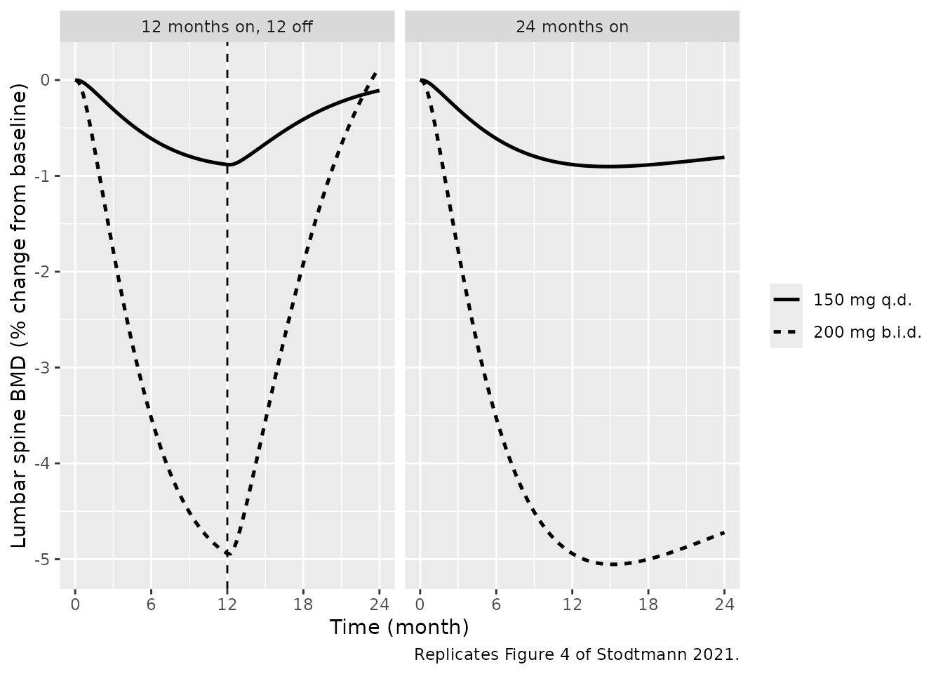
recovery <- fig4 |>
  dplyr::filter(scenario == "12 months on, 12 off", abs(month - 24) < 1e-6)
recovery |>
  dplyr::select(regimen, BMDlspct) |>
  dplyr::rename("Regimen" = regimen, "BMD change at month 24 (%)" = BMDlspct) |>
knitr::kable(digits = 2)| Regimen | BMD change at month 24 (%) |
|---|---|
| 150 mg q.d. | -0.11 |
| 200 mg b.i.d. | 0.14 |
Check 6: Figure 3, treatment sequences of the phase 3 program
sequences <- list(
  "plac/150QD/post" = list(start = c(0, 6, 12), dose = c(0, 150, 0)),
  "plac/200BID/post" = list(start = c(0, 6, 12), dose = c(0, 400, 0)),
  "150QD/150QD/post" = list(start = c(0, 12), dose = c(150, 0)),
  "200BID/200BID/post" = list(start = c(0, 12), dose = c(400, 0))
)
fig3 <- dplyr::bind_rows(lapply(names(sequences), function(nm) {
  s <- sequences[[nm]]
  simulate_sequence(s$start, s$dose, end_month = 36) |>
    dplyr::mutate(sequence = nm)
}))
fig3_long <- fig3 |>
  dplyr::select(sequence, month, BMD = BMDlspct, CTX = CTXchgpct, P1NP = P1NPchgpct) |>
  tidyr::pivot_longer(c(BMD, CTX, P1NP), names_to = "endpoint", values_to = "change") |>
  dplyr::mutate(sequence = factor(sequence, levels = names(sequences)),
                endpoint = factor(endpoint, levels = c("BMD", "CTX", "P1NP")))
ggplot(fig3_long, aes(month, change)) +
  geom_line(linewidth = 0.8) +
  geom_vline(xintercept = 12, linetype = "dashed") +
  facet_grid(endpoint ~ sequence, scales = "free_y") +
  scale_x_continuous(breaks = seq(0, 36, 6)) +
  labs(x = "Time (month)", y = "Change from baseline (%)",
       caption = "Replicates the model lines of Figure 3 of Stodtmann 2021.")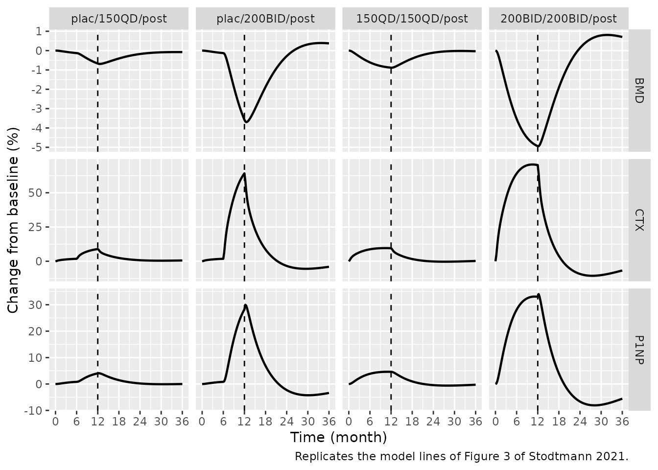
At the end of 12 months of 200 mg twice daily the model gives CTX and P1NP increases of about 70% and 33%, the level the Figure 3 model line and the EM-III / EM-IV data reach; the biomarkers return to baseline within about six months of stopping, BMD more slowly.
end_of_treatment <- fig3 |>
  dplyr::filter(abs(month - 12) < 1e-6) |>
  dplyr::select(sequence, BMDlspct, CTXchgpct, P1NPchgpct)
end_of_treatment |>
  dplyr::rename("Sequence" = sequence, "BMD (%)" = BMDlspct,
                "CTX (%)" = CTXchgpct, "P1NP (%)" = P1NPchgpct) |>
knitr::kable(digits = 1)| Sequence | BMD (%) | CTX (%) | P1NP (%) |
|---|---|---|---|
| plac/150QD/post | -0.7 | 8.9 | 4.0 |
| plac/200BID/post | -3.6 | 64.1 | 28.2 |
| 150QD/150QD/post | -0.9 | 9.5 | 4.6 |
| 200BID/200BID/post | -4.9 | 70.2 | 33.0 |
eot <- function(nm, col) end_of_treatment[[col]][end_of_treatment$sequence == nm]
stopifnot(
  # Figure 3 (right), month 12 of 200 mg b.i.d., read from the plot
  eot("200BID/200BID/post", "CTXchgpct") > 55, eot("200BID/200BID/post", "CTXchgpct") < 85,
  eot("200BID/200BID/post", "P1NPchgpct") > 20, eot("200BID/200BID/post", "P1NPchgpct") < 45,
  # Resorption rises more than formation, which is what drives BMD down
  eot("200BID/200BID/post", "CTXchgpct") > eot("200BID/200BID/post", "P1NPchgpct"),
  # Six months of treatment after placebo lose less BMD than twelve months
  eot("plac/200BID/post", "BMDlspct") > eot("200BID/200BID/post", "BMDlspct")
)
# Six months after stopping 200 mg b.i.d.: markers near baseline, BMD not yet
six_months_off <- fig3 |>
  dplyr::filter(sequence == "200BID/200BID/post", abs(month - 18) < 1e-6)
six_months_off[, c("BMDlspct", "CTXchgpct", "P1NPchgpct")]
#>    BMDlspct CTXchgpct P1NPchgpct
#> 1 -1.912322  3.876757   4.006426
stopifnot(
  abs(six_months_off$CTXchgpct) < 10,
  abs(six_months_off$P1NPchgpct) < 10,
  six_months_off$BMDlspct < -1
)
Check 7: Figure 2, response against E2 suppression at months 6 and 12
E2 suppression is 1 - e2 / 100, against the Riggs 2012
reference; the paper’s placebo observations sit at the ~5% suppression
this implies for the untreated 94.9 pg/mL.
fig2_doses <- seq(0, 600, by = 20)
fig2 <- dplyr::bind_rows(lapply(fig2_doses, function(d) {
  sim <- simulate_sequence(0, d, end_month = 12, by = 6)
  sim |>
    dplyr::filter(month %in% c(6, 12)) |>
    dplyr::transmute(month, suppression = 100 * (1 - e2 / 100),
                     BMD = BMDlspct, CTX = CTXchgpct, P1NP = P1NPchgpct)
}))
fig2 |>
  tidyr::pivot_longer(c(BMD, CTX, P1NP), names_to = "endpoint", values_to = "change") |>
  dplyr::mutate(month = paste("Month", month)) |>
  ggplot(aes(suppression, change)) +
  geom_line(linewidth = 0.8) +
  facet_grid(endpoint ~ month, scales = "free_y") +
  labs(x = "Estradiol suppression (%)", y = "Change from baseline (%)",
       caption = "Replicates the model lines of Figure 2 of Stodtmann 2021.")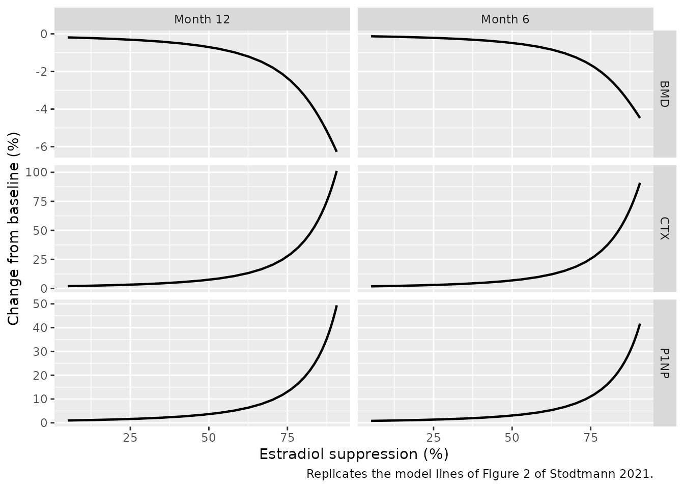
Assumptions and deviations
- E2 fraction reference. Stodtmann 2021 does not say how its predicted E2 was converted to the fraction that enters Riggs 2012 equation 6. The model uses E2 / 100 pg/mL, the “typical baseline E2 of ~100 pg/ml” Riggs 2012 uses to define its suppression categories. E2 relative to the untreated 94.9 pg/mL reproduces Table 3 markedly worse (Check 4), and the paper’s Figure 2 placebo points, at ~5% suppression, confirm the 100 pg/mL reference.
-
Printed Riggs 2012 values over code values. Where
Riggs 2012 prints a value and OpenBoneMin carries a different one, the
printed value is used, matching the paper’s statement that the model was
applied as published:
tgfbGAM0.075 (code 0.0374),tgfbactGAM0.045 (code 0.045273),E2scalePicB10.000012 (code 0.0000116832) andgamOB0.0739 (code 0.0793). Substituting the code’stgfbGAMorgamOBworsens the Table 3 agreement (Check 4). - Deterministic, typical value. No inter-individual variability and no residual error were reported; the paper describes population-level trends.
- Estrogen fraction applied instantaneously. The dose-E2 model is a steady-state relationship, so E2 and E change as a step when the daily dose changes. The 12-hour estrogen half-life of Riggs 2012 equation 1 is negligible against the months-long bone response.
- Menopause limb omitted. The age-driven estrogen decline of Riggs 2012 equation 1 describes the menopause transition and is switched off in OpenBoneMin by default; the population here is premenopausal, so it is not included.
- Inert OpenBoneMin components dropped. The denosumab, teriparatide and generic-drug PK compartments, the denosumab-specific and femoral-neck BMD states and the GFR-decline state are all inert unless dosed or switched on, and are not part of this model. Glomerular filtration is fixed at the OpenBoneMin baseline of 100 mL/min.
- P1NP as the formation marker. Riggs 2012 uses total osteoblasts relative to baseline as its bone-specific alkaline phosphatase surrogate; Stodtmann 2021 compares the same model quantity with P1NP, which was measured in the elagolix trials instead of BSAP.
- Residual shape difference beyond 12 months. Beyond the 12-month horizon of the validation data the packaged model reaches its BMD nadir around month 15 rather than about month 17 (Figure 4) and recovers slightly faster on continued treatment, so it under-predicts the published 24-month loss by about 0.1 (150 mg q.d.) and 0.25 (200 mg b.i.d.) percentage points (Check 4). None of the alternatives in Check 4 removes it, nor does a 28- or 30-day month; the cause is not identifiable from the paper.
Errata
-
Riggs 2012 BMD parameter labels. Riggs 2012 p 4
prints “kout,BMD (0.140 (unitless)) and gammaOC (0.00953 d^-1)”. The
units show the labels are swapped: an exponent is unitless and a rate
constant carries 1/day. OpenBoneMin confirms it, with
koutBMDls = 0.000397/h (= 0.00953 /day) andgamOCls = 0.14. The model uses the corrected assignment. The alternative OpenBoneMin set (koutBMDlsDEN,gamOClsDEN), fitted in the separate CKD analysis, reproduces Table 3 an order of magnitude worse (Check 4) and is not the set used here. -
Riggs 2012
gamOB0.0739 versus OpenBoneMin 0.0793. Two Riggs papers print 0.0739; the code’s 0.0793 looks like a digit transposition. The printed value is used (see above).