KRAS G12C covalent inhibitors (Stites 2018) • nlmixr2lib

library(nlmixr2lib)
library(rxode2)
library(dplyr)
library(tidyr)
library(ggplot2)
library(knitr)

What this paper contributes

Stites and Shaw (2018) take an existing mechanistic model of the Ras nucleotide-cycling network and ask a drug-development question with it: why do the two classes of covalent KRAS G12C inhibitor behave the way they do in cells, and which biochemical property would you optimise to make the weaker class work?

The two classes differ in where the compound ends up after it has bonded to the G12C cysteine.

Nucleotide-pocket inhibitors (NPIs) sit in the guanine-nucleotide pocket, so they can only bind KRAS G12C that is momentarily nucleotide-free.
Switch-II-pocket inhibitors (SIIPIs) sit in a separate allosteric pocket. They bind the GDP-bound (and nucleotide-free) mutant and prevent it from reloading GTP.

The model’s central structural claim is that covalent-inhibitor efficacy is turnover-limited. Because the bond is irreversible, the drug can only ever capture protein that passes through the bindable state before it is degraded, so the relevant quantity is a rate of capture competing against Ras protein turnover – not an affinity. The paper makes this explicit: these compounds have no Kd to assign, only an on-rate.

Two things follow, and both are reproduced below. First, adding protein turnover to the model changes nothing about oncogenic mutant signalling in the absence of drug (Figure 1) but completely changes the predicted drug dose response (Figure 2). Second, the properties that make a secondary mutation resistant to a SIIPI can make it more sensitive to an NPI (Figure 6) – so the two strategies are worth pursuing in parallel.

Provenance

The main text is short on equations by design: the Methods section says only that “the model is specified as a set of coupled, nonlinear, ordinary differential equations”, and Table 1 tabulates just the eleven parameters that are new in this paper. The rest of the network comes from the authors’ earlier Ras model (Stites 2007, Science 318:463-467).

That gap is closed completely by the article’s Supporting Information. The archive PSP4-7-342-s001.zip contains a folder Model Files with eleven MATLAB scripts and a Read_Me.pdf:

File	Role
`G12CDrugModel.m`	The 14 differential equations and the 34-element rate-constant vector
`RasG12C_inhibition.m`	Every parameter value, the initial conditions, and the steady-state driver
`RasG12C_inhibition_NT.m`	The same system with turnover switched off
`RasG12C_inhibition_timecourse.m`	Drug-free equilibration followed by drug addition
`GenerateFigure2.m` … `GenerateFigure6.m`	The exact scenario settings behind each published figure

Every value in inst/modeldb/therapeuticArea/Stites_2018_kras_g12c_qsp.R is transcribed from those files, cross-checked against Table 1 where Table 1 reports it. Nothing is supplied from outside those sources.

mod <- rxode2::rxode(readModelDb("Stites_2018_kras_g12c_qsp"))
cat(mod$description)
#> QSP. In vitro / in silico (human KRAS G12C mutant cancer cell network). Mechanistic 14-state model of the Ras nucleotide-cycling network -- GEF-catalysed exchange, GAP-accelerated and intrinsic GTP hydrolysis, nucleotide association and dissociation, effector binding, and first-order Ras protein production and degradation -- carrying both wild-type Ras (KRAS + NRAS + HRAS) and the KRAS G12C mutant, extended with the two classes of covalent G12C inhibitor. Nucleotide-pocket inhibitors (NPIs, e.g. SML-8-73-1) bind irreversibly to nucleotide-free G12C; switch-II-pocket inhibitors (SIIPIs, e.g. ARS-853 and Ostrem compound 12) bind irreversibly to GDP-bound and nucleotide-free G12C and block GTP loading. Both drug-bound forms remain subject to Ras degradation, which is what makes covalent-inhibitor efficacy turnover-limited. An optional GEF-loading arm lets Ras GEFs load an NPI into the nucleotide pocket in competition with GTP and GDP. Steady-state readouts are the fraction of total Ras in the GTP-bound state and the fraction of effector bound to RasGTP; secondary G12C mutations are simulated by scaling the intrinsic GTPase rate and the intrinsic nucleotide dissociation rates.

str(mod$population)
#> List of 7
#>  $ species      : chr "in silico (human KRAS G12C mutant cancer cell); parameterised from human and in vitro Ras biochemistry"
#>  $ n_subjects   : int 0
#>  $ n_studies    : int 0
#>  $ disease_state: chr "KRAS G12C mutant cancer (lung adenocarcinoma is the motivating indication)"
#>  $ dose_range   : chr "Covalent inhibitor concentrations of 0 to 1e-5 M (0 to 10 micromolar) were simulated; the published dose-respon"| __truncated__
#>  $ regions      : chr "Not applicable (no clinical study)"
#>  $ notes        : chr "No subjects were studied. This is a purely mechanistic model: the paper fits nothing and estimates nothing, and"| __truncated__

Source trace

Eleven parameters are printed in the paper itself; the remaining twenty-one are biochemical constants that appear only in the deposited code. Both were available when this model was built.

Model parameter	Value	Source in the paper	Source in the deposited code
`kdeg`	8e-6 /s	Table 1, `k deg`	`RasG12C_inhibition.m`: `kDeg=8e-6`
(derived `kpro_wt` + `kpro_mut`)	3.2e-12 M/s	Table 1, `k production`	`k(30)=k(29)WTRasTot`, `k(31)=k(29)MutTot`
`kon_drug` (NPI)	2e6 1/(M*s)	Table 1, `k on,NPI`	`GenerateFigure2.m`: `onrateNPI=2e6`
`kon_drug` (SIIPI cpd 12)	0.12 1/(M*s)	Table 1, `k on,SIIPI,12`	`GenerateFigure2.m`: `onrateSIIPI=.12`
`kon_drug` (SIIPI ARS-853)	76 1/(M*s)	Table 1, `k on,SIIPI,ARS`	`GenerateFigure2.m`: `onrateARS=76`
`mut_frac` / `wt_frac`	0.25 / 0.75	Table 1, `Percent_KRAS` 50 and `Percent_Mut` 50	`concs = [.25,.75,...]` in every driver
`scale_gtpase_g12c`	49/68 = 0.7206	Table 1, `Scalingfactor GTPase,G12C` = 72%	`mkint=(49/68)kint(1/changes(1))`
`scale_kd_eff_g12c`	67/56 = 1.196	Table 1, `Scalingfactor kdissG12C` = 120%	`mKd=(67/56)*Kd`
`gtp`	1.8e-4 M	Table 1, `GTP`	`GTP=180e-6`
`gdp`	1.8e-5 M	Table 1, `GDP`	`GDP=18e-6`
`gtot`, `efftot`	4e-7 M each	not printed	`GTot=4e-7`, `EffTot=4e-7`
`gef`, `gap`	2e-10, 6e-11 M	not printed	`GEF=(2e-10)*RTKfact`, `GAP=6e-11`
`kgtpase`	3.5e-4 /s	not printed	`kint=3.5e-4`
`kdiss_gdp`, `kdiss_gtp`	1.1e-4, 2.5e-4 /s	not printed	`kdissD`, `kdissT`
`kass_gdp`, `kass_gtp`	2.3e6, 2.2e6 1/(M*s)	not printed	`kassD`, `kassT`
`kcat_gap`, `km_gap`	5.4 /s, 2.3e-7 M	not printed	`kcat=5.4`, `Km=.23e-6/volscale`
`kcat_gef_gdp`	3.9 /s	not printed	`kD=3.9`
`km_gef_gdp`, `km_gef_gtp`	3.86e-4, 3e-4 M	not printed	`KmD`, `KmT` (before `/volscale`)
`kass_eff`, `kd_eff`	4.5e7 1/(M*s), 8e-8 M	not printed	`kassEff=4.5e7`, `Kd=80e-9`
`volscale`	250	not printed	`volscale=250`
ODE system (14 states)	–	described in prose only	`G12CDrugModel.m`, `dydt` vector

Two derived quantities are not free parameters and are recomputed inside model() exactly as the deposited code does: the reverse GEF catalytic constant is fixed by the Haldane relationship for the intrinsic nucleotide reactions (kT = kD * KmT * Haldane / KmD), and Ras production is set so that the drug-free steady state reproduces the specified cellular abundance (kpro = kdeg * total).

Simulation helpers

The paper’s readouts are steady-state quantities. The deposited driver reaches them by integrating a 10,000 s window repeatedly until the state stops moving; integrating once to a long horizon is equivalent and is what is done here. Ras turnover has a 24 h half-life, so 2e6 s is roughly sixteen half-lives.

Absolute tolerance is the one setting that matters: the states are molar concentrations of order 1e-7, so rxode2’s default atol would be looser than the quantities being resolved.

T_SS <- 2e6 # s, about 16 Ras half-lives
EV_SS <- rxode2::et(c(0, T_SS / 2, T_SS))

# Published dose grid (GenerateFigure2.m / GenerateFigure4.m / GenerateFigure5B.m)
DOSES <- c(
  0, 1e-10, 1e-9, 2e-9, 5e-9, 1e-8, 1.3e-8, 2e-8, 3e-8, 5e-8, 7e-8, 1e-7,
  1.3e-7, 2e-7, 3e-7, 5e-7, 7e-7, 1e-6, 1.3e-6, 2e-6, 3e-6, 5e-6, 7e-6, 1e-5
)

solve_scenarios <- function(pars, events = EV_SS) {
  s <- rxode2::rxSolve(
    mod, events,
    params = pars,
    atol = 1e-16, rtol = 1e-10, maxsteps = 1e6,
    returnType = "data.frame"
  )
  n <- nrow(pars)
  ntime <- nrow(s) / n
  stopifnot(ntime == length(unique(s$time)))
  # rxode2 returns one contiguous block of times per params row. Label the
  # blocks, then PROVE the labelling by checking that the free-drug state at
  # t = 0 is the dose that row asked for -- a mis-ordered block would show up
  # here rather than silently mislabel every curve downstream.
  s$scenario <- rep(seq_len(n), each = ntime)
  t0 <- s[s$time == 0, ]
  t0 <- t0[order(t0$scenario), ]
  if (!is.null(pars$npi0)) stopifnot(isTRUE(all.equal(t0$npi, rep_len(pars$npi0, n))))
  if (!is.null(pars$siipi0)) stopifnot(isTRUE(all.equal(t0$siipi, rep_len(pars$siipi0, n))))
  s
}

# Steady-state rows only, one per scenario.
steady_state <- function(pars, events = EV_SS) {
  s <- solve_scenarios(pars, events)
  out <- s[s$time == max(s$time), ]
  out[order(out$scenario), ]
}

# Every published dose response is plotted as a percentage of that scenario's
# own drug-free value (the `100*Eff(:,j)/Eff(1,j)` idiom of the MATLAB drivers).
pct_of_undosed <- function(x) 100 * x / x[1]

Structural verification

Before reproducing any figure, check the things that must be true of the ODE system itself. These are deterministic – there is no simulated cohort and no random number generation anywhere in this vignette – so the tolerances are as tight as the solver allows, and every one of them can go red.

Conservation laws

The network has four independent conserved quantities, and each one is a different transcription error caught. Total wild-type Ras and total mutant Ras are set by the production/degradation balance. Total effector is conserved because effector released from a degrading Ras:effector complex returns to the free pool. Total NPI and total SIIPI are conserved because drug released from a degrading drug-bound Ras likewise returns to the free pool – if the +r38, +r30 or +r32 terms were dropped the drug would silently disappear and every dose response would be too shallow.

cons <- steady_state(data.frame(npi0 = c(0, 3e-7, 0), siipi0 = c(0, 0, 3e-7)))

wt_total <- with(cons, ras_gdp + ras_gtp + ras_free + ras_gtp_eff)
mut_total <- with(cons, g12c_gdp + g12c_gtp + g12c_free + g12c_gtp_eff +
  g12c_gdp_siipi + g12c_free_siipi + g12c_npi)
eff_total <- with(cons, eff + ras_gtp_eff + g12c_gtp_eff)
npi_total <- with(cons, npi + g12c_npi)
siipi_total <- with(cons, siipi + g12c_gdp_siipi + g12c_free_siipi)

conservation <- tibble::tibble(
  Quantity = c(
    "Total wild-type Ras", "Total KRAS G12C", "Total effector",
    "Total NPI", "Total SIIPI"
  ),
  Expected = c(3e-7, 1e-7, 4e-7, 3e-7, 3e-7),
  `Worst relative error` = c(
    max(abs(wt_total - 3e-7)) / 3e-7,
    max(abs(mut_total - 1e-7)) / 1e-7,
    max(abs(eff_total - 4e-7)) / 4e-7,
    abs(npi_total[2] - 3e-7) / 3e-7,
    abs(siipi_total[3] - 3e-7) / 3e-7
  )
)
kable(conservation, digits = c(0, 10, 12))

Quantity	Expected	Worst relative error
Total wild-type Ras	3e-07	0
Total KRAS G12C	1e-07	0
Total effector	4e-07	0
Total NPI	3e-07	0
Total SIIPI	3e-07	0


# All five are algebraic identities of the ODE system, not fitted agreements.
stopifnot(all(conservation$`Worst relative error` < 1e-9))

Steady state actually reached

hold <- solve_scenarios(data.frame(siipi0 = c(0, 1e-6, 1e-5), kon_drug = 76))
mid <- hold[hold$time == T_SS / 2, ]
end <- hold[hold$time == T_SS, ]
mid <- mid[order(mid$scenario), ]
end <- end[order(end$scenario), ]
drift <- max(abs(end$frac_eff_bound - mid$frac_eff_bound) / mid$frac_eff_bound)
cat(sprintf(
  "Largest change in Ras signal between t = %.0e s and t = %.0e s: %.2e (relative)\n",
  T_SS / 2, T_SS, drift
))
#> Largest change in Ras signal between t = 1e+06 s and t = 2e+06 s: 4.44e-10 (relative)
# Eight further half-lives change the answer by less than one part in 1e9.
stopifnot(drift < 1e-9)

Dimensional check

The two second-order nucleotide association constants enter the ODEs only after being multiplied by the cellular nucleotide abundance, which turns them into the pseudo-first-order constants the system actually uses. Confirming the magnitude is worthwhile because it is what makes nucleotide-free Ras vanishingly rare, and that rarity is the paper’s whole explanation for why NPIs underperform.

free <- steady_state(data.frame(npi0 = 0, siipi0 = 0))
cat(sprintf(
  "kass_gdp * [GDP] = %.1f /s and kass_gtp * [GTP] = %.1f /s, against nucleotide
dissociation rates of 1.1e-4 and 2.5e-4 /s.\n",
  2.3e6 * 1.8e-5, 2.2e6 * 1.8e-4
))
#> kass_gdp * [GDP] = 41.4 /s and kass_gtp * [GTP] = 396.0 /s, against nucleotide
#> dissociation rates of 1.1e-4 and 2.5e-4 /s.
cat(sprintf(
  "At the drug-free steady state nucleotide-free KRAS G12C is %.2e M, which is
%.1e of the GDP-bound mutant pool.\n",
  free$g12c_free, free$g12c_free / free$g12c_gdp
))
#> At the drug-free steady state nucleotide-free KRAS G12C is 1.93e-14 M, which is
#> 5.5e-07 of the GDP-bound mutant pool.
stopifnot(free$g12c_free / free$g12c_gdp < 1e-5)

Figure 1: turnover does not change drug-free signalling

Figure 1b and 1c make the negative control explicit: adding protein production and degradation to the 2007 model leaves the predicted steady-state Ras signal essentially unchanged, whether the signal is raised by an oncogenic mutation (1b) or by loss of the tumour suppressor NF1 (1c). That is what licenses the authors to reuse the earlier model’s parameter estimates.

The deposited archive ships drivers for Figures 2 through 6 only, so the G12V, G12D and F28L columns of Figure 1b – whose mutant scaling factors come from the 2007 paper, which was not available when this model was built – cannot be reproduced here. The wild-type and G12C columns can.

turnover <- steady_state(data.frame(
  mut_frac = c(0, 0.25, 0, 0.25),
  wt_frac = c(1, 0.75, 1, 0.75),
  kdeg = c(8e-6, 8e-6, 0, 0)
))
fig1b <- tibble::tibble(
  Network = c("All wild-type Ras", "25% KRAS G12C", "All wild-type Ras", "25% KRAS G12C"),
  Model = c("with turnover", "with turnover", "no turnover", "no turnover"),
  `Fraction of Ras bound to GTP` = turnover$frac_ras_active,
  `Fraction of effector bound` = turnover$frac_eff_bound
)
kable(fig1b, digits = 4)

Network	Model	Fraction of Ras bound to GTP	Fraction of effector bound
All wild-type Ras	with turnover	0.0209	0.0174
25% KRAS G12C	with turnover	0.2749	0.2142
All wild-type Ras	no turnover	0.0202	0.0168
25% KRAS G12C	no turnover	0.2722	0.2122


# The paper's claim is that the two model versions agree, not that they are
# bit-identical. Realised: 3.26% relative on the all-wild-type network (an
# absolute gap of 0.0007 on a 0.021 signal) and 0.98% on the G12C network
# (0.0027 on 0.275) -- indistinguishable on the axes of Figure 1b. The
# absolute bound is the one that matches the published claim, since the
# wild-type signal is small; both are held. A mis-transcribed production or
# degradation term moves these by tens of percent, not tenths.
abs_gap <- abs(turnover$frac_ras_active[1:2] - turnover$frac_ras_active[3:4])
rel_gap <- abs_gap / turnover$frac_ras_active[1:2]
cat(sprintf(
  "Largest turnover-vs-no-turnover discrepancy: %.2f%% relative, %.4f absolute\n",
  100 * max(rel_gap), max(abs_gap)
))
#> Largest turnover-vs-no-turnover discrepancy: 3.26% relative, 0.0027 absolute
stopifnot(max(rel_gap) < 0.05, max(abs_gap) < 0.005)

# ... and the G12C mutant raises Ras signalling many-fold over wild type.
stopifnot(turnover$frac_ras_active[2] / turnover$frac_ras_active[1] > 10)

gap_levels <- c(1, 0.75, 0.5, 0.25, 0)
fig1c <- steady_state(data.frame(gap = 6e-11 * gap_levels))
fig1c_nt <- steady_state(data.frame(gap = 6e-11 * gap_levels, kdeg = 0))

fig1c_tab <- tibble::tibble(
  `Basal GAP activity remaining` = paste0(100 * gap_levels, "%"),
  `RasGTP, with turnover` = fig1c$frac_ras_active,
  `RasGTP, no turnover` = fig1c_nt$frac_ras_active
)
kable(fig1c_tab, digits = 4)

Basal GAP activity remaining	RasGTP, with turnover	RasGTP, no turnover
100%	0.2749	0.2722
75%	0.3117	0.3085
50%	0.3717	0.3680
25%	0.4672	0.4636
0%	0.6021	0.5994


# GAP is the negative regulator: losing it must raise RasGTP monotonically,
# and losing all of it must move the signal substantially (0.275 -> 0.602).
stopifnot(all(diff(fig1c$frac_ras_active) > 0))
stopifnot(fig1c$frac_ras_active[5] / fig1c$frac_ras_active[1] > 2)
# And, again, turnover must not matter. Realised gaps 0.4-1.0% relative across
# the five GAP levels, all under 0.004 absolute.
stopifnot(max(abs(fig1c$frac_ras_active - fig1c_nt$frac_ras_active) /
  fig1c$frac_ras_active) < 0.05)
stopifnot(max(abs(fig1c$frac_ras_active - fig1c_nt$frac_ras_active)) < 0.005)

Figure 2: turnover changes the drug dose response completely

Now the positive result. Each compound is simulated over the published 24-point dose grid, first with turnover and then without. Without turnover the system is closed: the drug simply consumes mutant protein until either the drug or the mutant runs out, and all three compounds land on the same curve regardless of on-rate. With turnover, freshly produced drug-free mutant keeps arriving, and the compounds separate entirely by how fast they can capture it.

npi <- steady_state(data.frame(npi0 = DOSES, siipi0 = 0, kon_drug = 2e6))
siipi12 <- steady_state(data.frame(npi0 = 0, siipi0 = DOSES, kon_drug = 0.12))
ars853 <- steady_state(data.frame(npi0 = 0, siipi0 = DOSES, kon_drug = 76))

# No-turnover arm: RasG12C_inhibition_NT.m sets kdeg (and both production
# rates) to zero and reduces the mutant pool by the drug already consumed,
# clamped at zero -- the drug itself is then not given as a free species.
nt <- steady_state(data.frame(
  mut_frac = pmax(0, 0.25 - DOSES / 4e-7),
  wt_frac = 0.75, kdeg = 0, npi0 = 0, siipi0 = 0
))

fig2 <- bind_rows(
  tibble::tibble(dose = DOSES, signal = pct_of_undosed(npi$frac_eff_bound),
                 series = "NPI, with turnover"),
  tibble::tibble(dose = DOSES, signal = pct_of_undosed(siipi12$frac_eff_bound),
                 series = "SIIPI (compound 12), with turnover"),
  tibble::tibble(dose = DOSES, signal = pct_of_undosed(ars853$frac_eff_bound),
                 series = "ARS-853 SIIPI, with turnover"),
  tibble::tibble(dose = DOSES, signal = pct_of_undosed(nt$frac_eff_bound),
                 series = "any inhibitor, no turnover")
)

ggplot(filter(fig2, dose > 0), aes(dose, signal, colour = series, linetype = series)) +
  geom_line(linewidth = 0.8) +
  scale_x_log10(limits = c(1e-9, 1e-5)) +
  scale_linetype_manual(values = c(1, 1, 1, 2)) +
  coord_cartesian(ylim = c(0, 105)) +
  labs(
    x = "drug concentration [M]", y = "Ras signal intensity (% of drug-free)",
    colour = NULL, linetype = NULL,
    title = "Replicates Figure 2c of Stites and Shaw (2018)"
  ) +
  theme_bw() +
  theme(legend.position = "bottom") +
  guides(colour = guide_legend(nrow = 2), linetype = guide_legend(nrow = 2))
#> Warning: Removed 4 rows containing missing values or values outside the scale range
#> (`geom_line()`).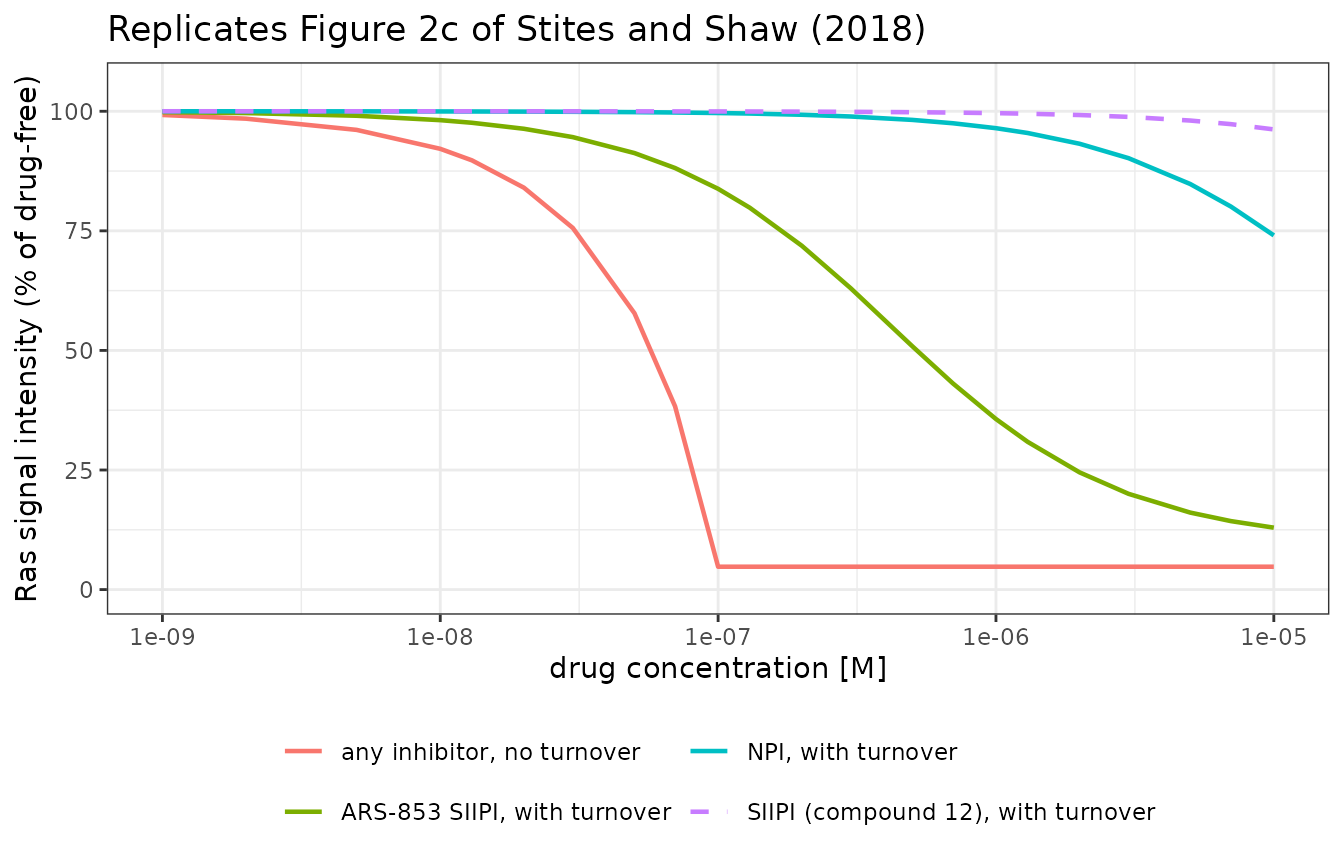

fig2_tab <- tibble::tibble(
  `Drug concentration (M)` = DOSES,
  `NPI` = pct_of_undosed(npi$frac_eff_bound),
  `SIIPI cpd 12` = pct_of_undosed(siipi12$frac_eff_bound),
  `ARS-853` = pct_of_undosed(ars853$frac_eff_bound),
  `No turnover` = pct_of_undosed(nt$frac_eff_bound)
) |>
  filter(`Drug concentration (M)` %in% c(0, 1e-8, 1e-7, 3e-7, 1e-6, 3e-6, 1e-5))
kable(fig2_tab, digits = 1)

NPI	SIIPI cpd 12	ARS-853	No turnover
100.0	100.0	100.0	100.0
100.0	100.0	98.1	92.1
99.6	100.0	83.8	4.8
98.9	99.9	63.0	4.8
96.5	99.6	35.7	4.8
90.2	98.8	20.0	4.8
74.1	96.2	12.9	4.8

Four features of the published panel are checked numerically.

at <- function(v, d) v[match(d, DOSES)]

# 1. The no-turnover curve collapses to a floor once the drug exceeds the
#    mutant pool, which is 25% of 4e-7 M, i.e. 1e-7 M. The floor sits near 5%
#    of the drug-free signal. Read off Figure 2c: the dashed grey line
#    flattens just past 1e-7 M at about 5.
nt_pct <- pct_of_undosed(nt$frac_eff_bound)
cat(sprintf("No-turnover floor: %.1f%%, first reached at %.1e M\n",
            min(nt_pct), DOSES[which(nt_pct <= min(nt_pct) * 1.001)[1]]))
#> No-turnover floor: 4.8%, first reached at 1.0e-07 M
stopifnot(abs(min(nt_pct) - 5) < 1.5)
stopifnot(DOSES[which(nt_pct <= min(nt_pct) * 1.001)[1]] <= 2e-7)

# 2. ARS-853 with turnover reaches about 13% of the drug-free signal at 1e-5 M
#    (Figure 2c, black curve endpoint).
ars_pct <- pct_of_undosed(ars853$frac_eff_bound)
cat(sprintf("ARS-853 at 1e-5 M: %.1f%% of drug-free signal\n", at(ars_pct, 1e-5)))
#> ARS-853 at 1e-5 M: 12.9% of drug-free signal
stopifnot(abs(at(ars_pct, 1e-5) - 13) < 2)

# 3. ARS-853 crosses 50% inhibition in the sub-micromolar range, which is what
#    the text describes as "the low micromolar range, with ~50% of Ras
#    inhibition occurring at 1 microM".
ic50 <- approx(ars_pct, DOSES, xout = 50)$y
cat(sprintf("ARS-853 concentration for 50%% of drug-free signal: %.2e M\n", ic50))
#> ARS-853 concentration for 50% of drug-free signal: 5.22e-07 M
stopifnot(ic50 > 1e-7, ic50 < 2e-6)

# 4. Turnover is what separates the compounds. Without it all three are the
#    same curve; with it, ARS-853 (on-rate 76) is far ahead of compound 12
#    (on-rate 0.12), which differ ONLY in kon_drug.
stopifnot(at(ars_pct, 1e-5) < at(pct_of_undosed(siipi12$frac_eff_bound), 1e-5) / 3)

The NPI and compound-12 SIIPI curves are the one place where this reproduction disagrees with the published panel; see Assumptions and deviations. The disagreement is a swap of the two, not a difference in values.

Figure 3: GEF activity modulates inhibition

Lito et al. showed that activating EGFR delays ARS-853 inhibition and inhibiting EGFR speeds it up – a result widely read as surprising, because oncogenic Ras was assumed to be GEF-independent. The model reproduces it without modification: EGFR activity is represented simply by scaling the basally active GEF pool.

Panel (a) is a time course. The system is first brought to its drug-free steady state and only then is the inhibitor allowed to engage, which is exactly what RasG12C_inhibition_timecourse.m does by equilibrating with the drug states at zero before setting them. Here the model’s tburn parameter holds every covalent binding reaction off until the burn-in is complete.

TBURN <- T_SS
EV_TC <- rxode2::et(sort(unique(c(
  seq(0, TBURN, length.out = 60),
  TBURN + seq(0, 10 * 3600, length.out = 150)
))))

tc <- solve_scenarios(
  data.frame(npi0 = 0, siipi0 = 1e-5, kon_drug = 76, tburn = TBURN,
             rtkfact = c(1, 10, 0.1)),
  events = EV_TC
)
tc_lab <- c("basal GEF", "10x GEF (RTK activation)", "0.1x GEF (RTK inhibition)")
tc_post <- tc |>
  filter(time >= TBURN) |>
  mutate(hours = (time - TBURN) / 3600, condition = tc_lab[scenario]) |>
  group_by(scenario) |>
  mutate(signal = 100 * total_rasgtp / total_rasgtp[1]) |>
  ungroup()

ggplot(tc_post, aes(hours, signal, colour = condition)) +
  geom_line(linewidth = 0.8) +
  labs(x = "time after ARS-853 addition (h)", y = "Ras signal (% of pre-dose)",
       colour = NULL, title = "Replicates Figure 3a of Stites and Shaw (2018)") +
  theme_bw() + theme(legend.position = "bottom")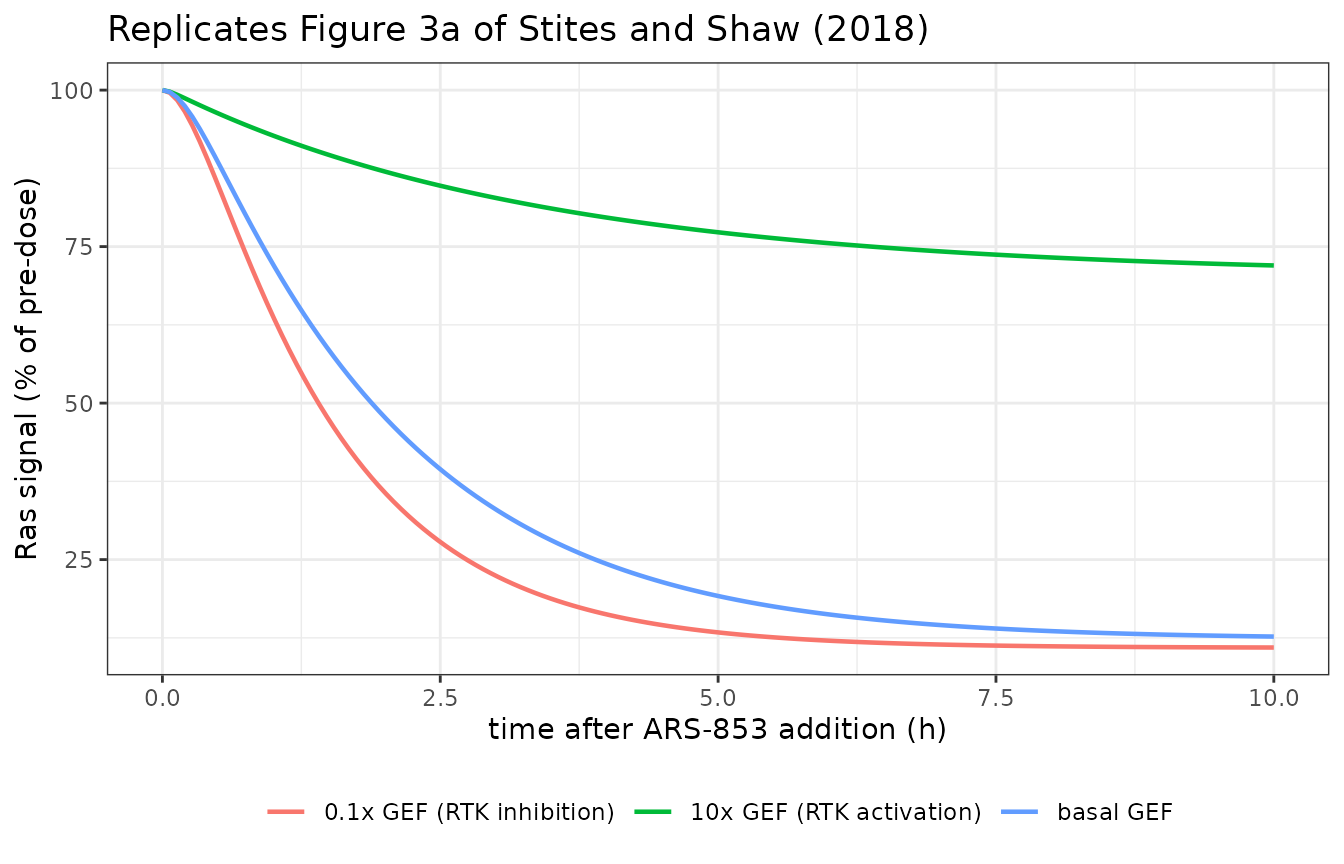

# Time to reach a given fraction of the pre-dose signal. Under 10x GEF the
# inhibition never reaches 50% inside the 10 h window Figure 3a plots (the
# green curve plateaus near 70%), so the 25%-inhibition mark is the deepest
# level that is defined for all three arms and is what the ordering gate uses.
time_to <- function(hours, signal, pct) {
  j <- which(signal <= pct)[1]
  if (is.na(j)) NA_real_ else hours[j]
}
tc_summary <- tc_post |>
  group_by(condition) |>
  summarise(
    `Pre-dose RasGTP (M)` = first(total_rasgtp),
    `Signal at 10 h (% of pre-dose)` = last(signal),
    `Hours to 25% inhibition` = time_to(hours, signal, 75),
    `Hours to 50% inhibition` = time_to(hours, signal, 50),
    .groups = "drop"
  ) |>
  arrange(match(condition, tc_lab))
kable(tc_summary, digits = c(0, 10, 1, 2, 2))

condition	Pre-dose RasGTP (M)	Signal at 10 h (% of pre-dose)	Hours to 25% inhibition	Hours to 50% inhibition
basal GEF	1.10e-07	12.7	0.94	1.95
10x GEF (RTK activation)	3.07e-07	72.0	6.44	NA
0.1x GEF (RTK inhibition)	4.30e-08	11.0	0.74	1.41


t25 <- tc_summary$`Hours to 25% inhibition`
s10 <- tc_summary$`Signal at 10 h (% of pre-dose)`
# This gate would be vacuous if an arm had failed to reach the mark at all.
stopifnot(!anyNA(t25))
# Raising GEF activity DELAYS inhibition; lowering it SPEEDS inhibition, by
# both the kinetic measure and the 10 h endpoint. This is the ordering Lito
# et al. measured and the paper set out to reproduce.
stopifnot(t25[2] > t25[1], t25[3] < t25[1])
stopifnot(s10[2] > s10[1], s10[3] < s10[1])
# Raising GEF activity also raises the pre-dose Ras signal itself (Figure 3a,
# right panel), which is the mechanism behind the delay.
stopifnot(tc_summary$`Pre-dose RasGTP (M)`[2] > tc_summary$`Pre-dose RasGTP (M)`[1])
stopifnot(tc_summary$`Pre-dose RasGTP (M)`[3] < tc_summary$`Pre-dose RasGTP (M)`[1])

Panels (c) and (d) are the corresponding steady-state dose responses.

rtk_levels <- c(1, 5, 0.2)
rtk_lab <- c("basal GEF", "5x GEF (RTK activation)", "0.2x GEF (RTK inhibition)")
fig3cd <- lapply(seq_along(rtk_levels), function(i) {
  v <- steady_state(data.frame(npi0 = 0, siipi0 = DOSES, kon_drug = 76,
                               rtkfact = rtk_levels[i]))
  tibble::tibble(dose = DOSES, condition = rtk_lab[i],
                 signal = pct_of_undosed(v$frac_ras_active),
                 rasgtp = v$total_rasgtp)
}) |> bind_rows()

ggplot(filter(fig3cd, dose > 0), aes(dose, signal, colour = condition)) +
  geom_line(linewidth = 0.8) +
  scale_x_log10(limits = c(1e-8, 1e-5)) +
  coord_cartesian(ylim = c(0, 100)) +
  labs(x = "ARS-853 concentration [M]", y = "Ras signal (% of drug-free)",
       colour = NULL, title = "Replicates Figure 3c of Stites and Shaw (2018)") +
  theme_bw() + theme(legend.position = "bottom")
#> Warning: Removed 12 rows containing missing values or values outside the scale range
#> (`geom_line()`).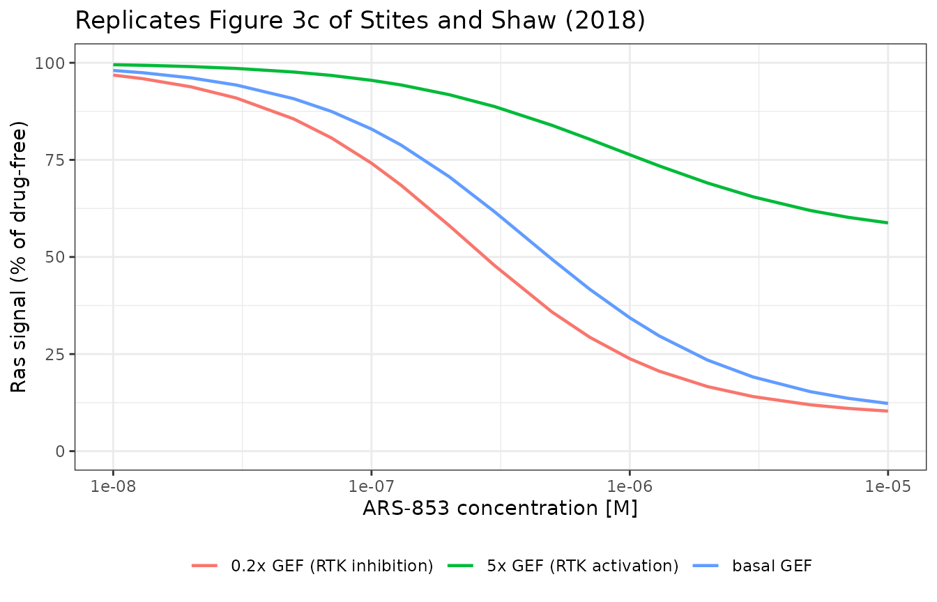

conc_for <- function(cond, pct) {
  d <- filter(fig3cd, condition == cond)
  if (nrow(d) == 0L) stop("no rows for condition '", cond, "'")
  approx(d$signal, d$dose, xout = pct)$y
}
fig3_tab <- tibble::tibble(
  Condition = rtk_lab,
  `Concentration for 75% signal (M)` = vapply(rtk_lab, conc_for, numeric(1), pct = 75),
  `Concentration for 50% signal (M)` = vapply(rtk_lab, conc_for, numeric(1), pct = 50),
  `Signal at 1e-5 M (%)` = vapply(rtk_lab, function(c1) {
    d <- filter(fig3cd, condition == c1)
    v <- d$signal[d$dose == 1e-5]
    if (length(v) != 1L) stop("no unique 1e-5 M row for '", c1, "'")
    v
  }, numeric(1))
)
kable(fig3_tab, digits = c(0, 10, 10, 1))

Condition	Concentration for 75% signal (M)	Concentration for 50% signal (M)	Signal at 1e-5 M (%)
basal GEF	1.6280e-07	4.903e-07	12.3
5x GEF (RTK activation)	1.1385e-06	NA	58.8
0.2x GEF (RTK inhibition)	9.6000e-08	2.783e-07	10.3


# Under 5x GEF the dose response never reaches 50% anywhere on the published
# grid (it bottoms out near 59%), so that column is NA there by construction
# and the 25%-inhibition mark is the deepest level defined for all three arms.
shift <- fig3_tab$`Concentration for 75% signal (M)`
stopifnot(!anyNA(shift))
# The dose response shifts RIGHT under GEF activation and LEFT under GEF
# inhibition -- the paper's Figure 3b/3c claim -- by both the potency shift
# and the endpoint at the top of the grid.
stopifnot(shift[2] > shift[1], shift[3] < shift[1])
stopifnot(fig3_tab$`Signal at 1e-5 M (%)`[2] > fig3_tab$`Signal at 1e-5 M (%)`[1])
stopifnot(fig3_tab$`Signal at 1e-5 M (%)`[3] < fig3_tab$`Signal at 1e-5 M (%)`[1])

Figure 4: secondary mutations blunt ARS-853

Lito et al. engineered KRAS alleles carrying G12C plus a second mutation that either impairs GTPase activity (A59G, Q61L, Y64A) or accelerates nucleotide exchange (Y40A, N116H, A146V), and showed both classes reduce ARS-853 sensitivity. Both are one-parameter changes in this model.

mut_grid <- list(
  list(lab = "KRAS G12C", g = 1, c = 1),
  list(lab = "10x slower GTPase", g = 10, c = 1),
  list(lab = "100x slower GTPase", g = 100, c = 1),
  list(lab = "10x faster cycling", g = 1, c = 10),
  list(lab = "100x faster cycling", g = 1, c = 100)
)
fig4 <- lapply(mut_grid, function(m) {
  v <- steady_state(data.frame(npi0 = 0, siipi0 = DOSES, kon_drug = 76,
                               fold_gtpase_impair = m$g, fold_cycling = m$c))
  tibble::tibble(dose = DOSES, mutant = m$lab,
                 signal = pct_of_undosed(v$frac_eff_bound))
}) |> bind_rows() |>
  mutate(mutant = factor(mutant, levels = vapply(mut_grid, `[[`, character(1), "lab")))

ggplot(filter(fig4, dose > 0), aes(dose, signal, colour = mutant)) +
  geom_line(linewidth = 0.8) +
  scale_x_log10(limits = c(1e-8, 1e-5)) +
  coord_cartesian(ylim = c(0, 100)) +
  labs(x = "ARS-853 concentration [M]", y = "Ras signal (% of drug-free)",
       colour = NULL, title = "Replicates Figure 4a and 4b of Stites and Shaw (2018)") +
  theme_bw() + theme(legend.position = "bottom")
#> Warning: Removed 20 rows containing missing values or values outside the scale range
#> (`geom_line()`).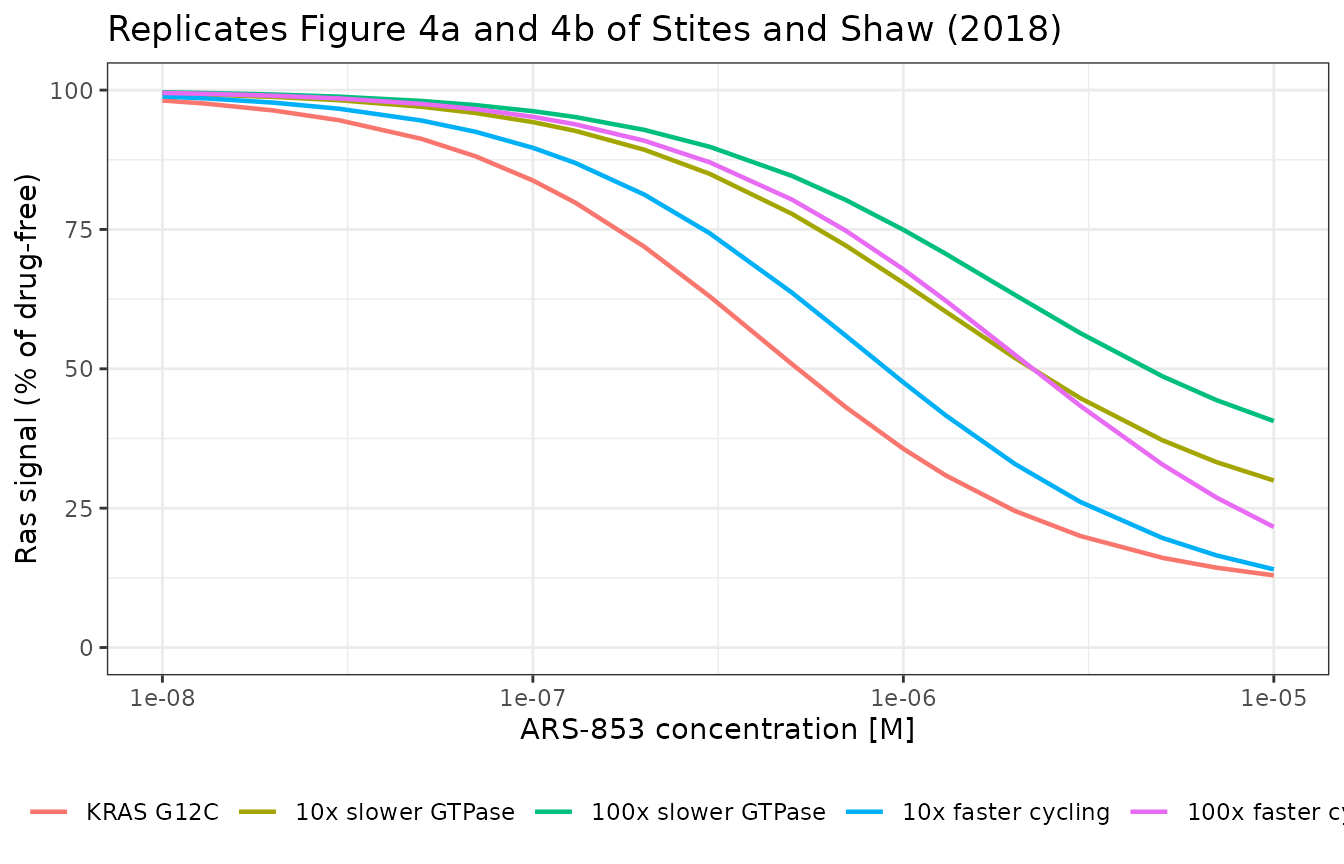

fig4_tab <- fig4 |>
  filter(dose == 1e-5) |>
  select(Mutant = mutant, `Signal at 1e-5 M ARS-853 (%)` = signal)
kable(fig4_tab, digits = 1)

Mutant	Signal at 1e-5 M ARS-853 (%)
KRAS G12C	12.9
10x slower GTPase	30.0
100x slower GTPase	40.6
10x faster cycling	14.0
100x faster cycling	21.6


s4 <- fig4_tab$`Signal at 1e-5 M ARS-853 (%)`
# Every secondary mutation leaves MORE residual signal than plain G12C, and the
# effect grows with the severity of the defect -- both directions the paper
# reports, in both mechanism classes.
stopifnot(all(s4[-1] > s4[1]))
stopifnot(s4[3] > s4[2], s4[5] > s4[4])

Figure 5: what would make an NPI work

An NPI can only bind mutant Ras whose pocket is momentarily empty, and the dimensional check above showed that state is about five parts in ten million of the mutant pool. The paper asks two questions: could a faster on-rate rescue the NPI, and could Ras GEFs be recruited to load the drug into the pocket?

onrate_mult <- c(0.1, 1, 10, 100, 1000)
fig5a <- lapply(onrate_mult, function(m) {
  v <- steady_state(data.frame(npi0 = DOSES, siipi0 = 0, kon_drug = 2e6 * m))
  tibble::tibble(dose = DOSES, on_rate = sprintf("%gx baseline", m),
                 signal = pct_of_undosed(v$frac_eff_bound))
}) |> bind_rows() |>
  mutate(on_rate = factor(on_rate, levels = sprintf("%gx baseline", onrate_mult)))

ggplot(filter(fig5a, dose > 0), aes(dose, signal, colour = on_rate)) +
  geom_line(linewidth = 0.8) +
  scale_x_log10() +
  coord_cartesian(ylim = c(0, 105)) +
  labs(x = "NPI concentration [M]", y = "Ras signal (% of drug-free)",
       colour = "NPI on-rate",
       title = "Replicates Figure 5a of Stites and Shaw (2018)") +
  theme_bw() + theme(legend.position = "bottom")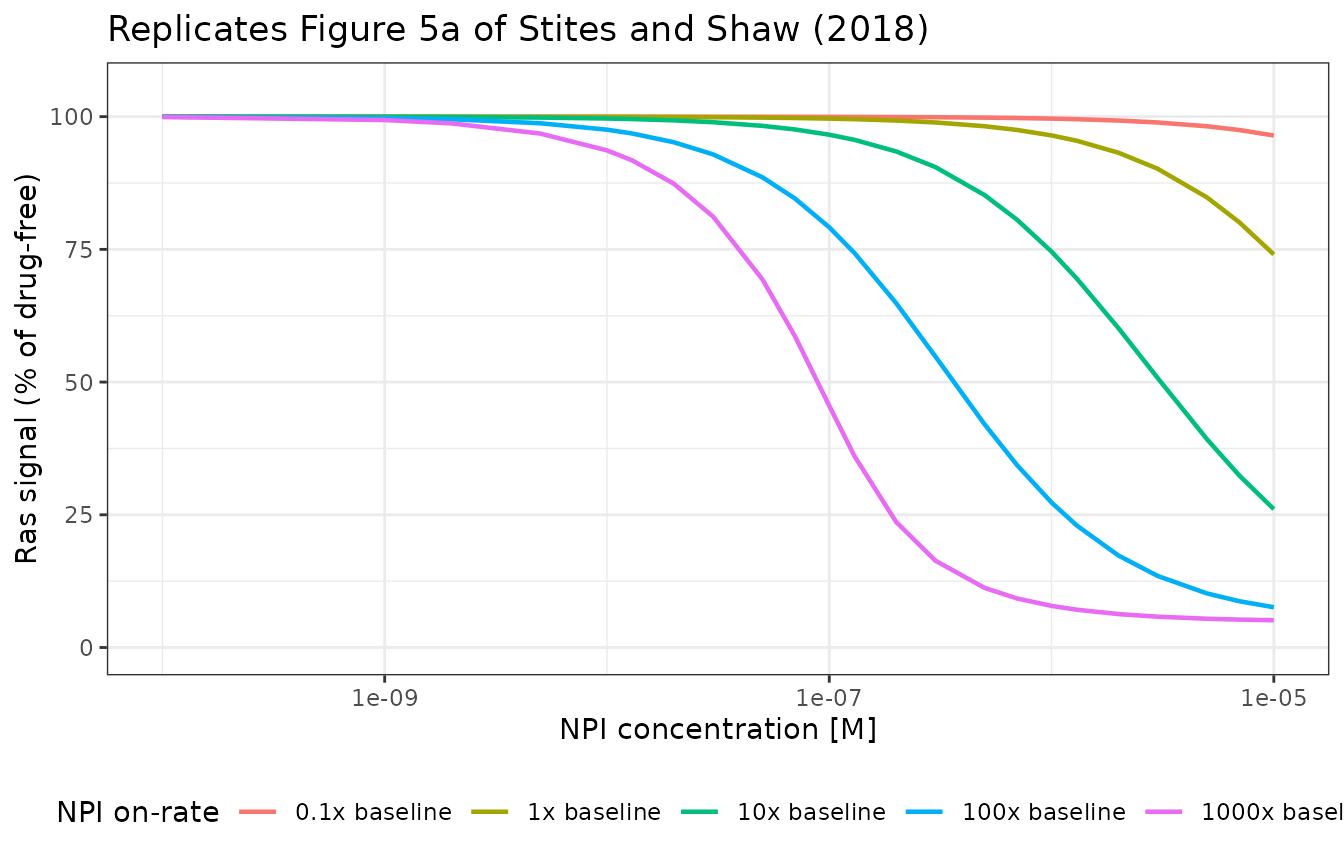

gefload_levels <- c(0, 1, 10, 100)
gefload_lab <- c("no GEF loading", "GEF loads NPI proportionally",
                 "GEF favours NPI 10x", "GEF favours NPI 100x")
fig5b <- lapply(seq_along(gefload_levels), function(i) {
  v <- steady_state(data.frame(npi0 = DOSES, siipi0 = 0, kon_drug = 2e6,
                               gefload = gefload_levels[i]))
  tibble::tibble(dose = DOSES, loading = gefload_lab[i],
                 signal = pct_of_undosed(v$frac_eff_bound))
}) |> bind_rows() |>
  mutate(loading = factor(loading, levels = gefload_lab))

ggplot(filter(fig5b, dose > 0), aes(dose, signal, colour = loading)) +
  geom_line(linewidth = 0.8) +
  scale_x_log10() +
  coord_cartesian(ylim = c(0, 105)) +
  labs(x = "NPI concentration [M]", y = "Ras signal (% of drug-free)",
       colour = NULL,
       title = "Replicates Figure 5b of Stites and Shaw (2018)") +
  theme_bw() + theme(legend.position = "bottom")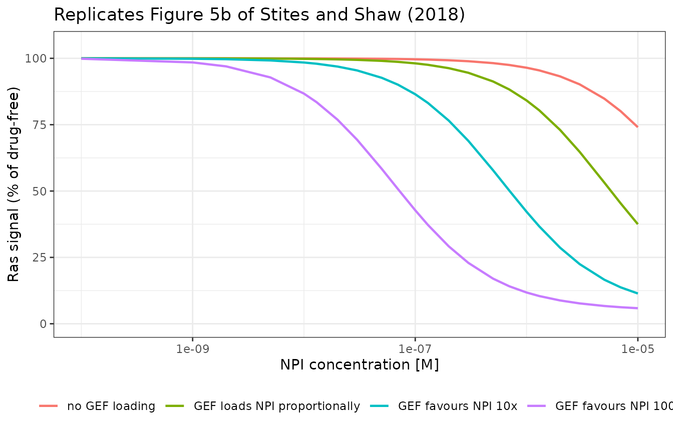

end_of <- function(df, col) {
  out <- vapply(
    levels(df[[col]]),
    function(k) {
      v <- df$signal[df[[col]] == k & df$dose == 1e-5]
      if (length(v) != 1L) stop("no unique 1e-5 M row for '", k, "'")
      v
    },
    numeric(1)
  )
  out
}
fig5_tab <- tibble::tibble(
  `NPI on-rate` = levels(fig5a$on_rate),
  `Signal at 1e-5 M (%)` = end_of(fig5a, "on_rate")
)
kable(fig5_tab, digits = 1)

NPI on-rate	Signal at 1e-5 M (%)
0.1x baseline	96.4
1x baseline	74.1
10x baseline	26.1
100x baseline	7.6
1000x baseline	5.1

fig5b_tab <- tibble::tibble(
  `GEF loading` = levels(fig5b$loading),
  `Signal at 1e-5 M (%)` = end_of(fig5b, "loading")
)
kable(fig5b_tab, digits = 1)

GEF loading	Signal at 1e-5 M (%)
no GEF loading	74.1
GEF loads NPI proportionally	37.5
GEF favours NPI 10x	11.4
GEF favours NPI 100x	5.9


# A faster on-rate monotonically improves the NPI, and so does GEF loading --
# the paper's two proposed optimisation routes.
stopifnot(all(diff(fig5_tab$`Signal at 1e-5 M (%)`) < 0))
stopifnot(all(diff(fig5b_tab$`Signal at 1e-5 M (%)`) < 0))

# The paper's quantitative claim about the optimised NPI: "the predicted levels
# of optimized (GEF-facilitated) NPI needed to inhibit 50% of the Ras signal
# were on the order of 1 microM, much smaller than the near mM levels of
# nucleotide" -- checked at the 10x GEF-favouring setting.
onpi10 <- filter(fig5b, loading == "GEF favours NPI 10x")
onpi_ic50 <- approx(onpi10$signal, onpi10$dose, xout = 50)$y
cat(sprintf("GEF-facilitated NPI concentration for 50%% signal: %.2e M\n", onpi_ic50))
#> GEF-facilitated NPI concentration for 50% signal: 7.07e-07 M
stopifnot(onpi_ic50 > 1e-7, onpi_ic50 < 1e-5)

Figure 6: the better inhibitor can change with resistance

This is the paper’s payoff. An optimised NPI (“oNPI”, modelled as GEF loading favouring the drug fourfold over nucleotide) is compared against ARS-853 for plain KRAS G12C and for each of the three resistance mechanisms.

fig6_cases <- list(
  list(lab = "KRAS G12C", g = 1, c = 1, r = 1),
  list(lab = "+ 100x faster cycling", g = 1, c = 100, r = 1),
  list(lab = "+ 100x slower GTPase", g = 100, c = 1, r = 1),
  list(lab = "+ 5x GEF (RTK activation)", g = 1, c = 1, r = 5)
)
fig6 <- lapply(fig6_cases, function(k) {
  sii <- steady_state(data.frame(npi0 = 0, siipi0 = DOSES, kon_drug = 76,
                                 gefload = 0, fold_gtpase_impair = k$g,
                                 fold_cycling = k$c, rtkfact = k$r))
  onp <- steady_state(data.frame(npi0 = DOSES, siipi0 = 0, kon_drug = 2e6,
                                 gefload = 4, fold_gtpase_impair = k$g,
                                 fold_cycling = k$c, rtkfact = k$r))
  bind_rows(
    tibble::tibble(dose = DOSES, case = k$lab, drug = "SIIPI (ARS-853)",
                   signal = pct_of_undosed(sii$frac_eff_bound)),
    tibble::tibble(dose = DOSES, case = k$lab, drug = "oNPI (GEF-facilitated)",
                   signal = pct_of_undosed(onp$frac_eff_bound))
  )
}) |> bind_rows() |>
  mutate(case = factor(case, levels = vapply(fig6_cases, `[[`, character(1), "lab")))

ggplot(filter(fig6, dose > 0), aes(dose, signal, colour = drug)) +
  geom_line(linewidth = 0.8) +
  facet_wrap(~case, nrow = 2) +
  scale_x_log10(limits = c(1e-8, 1e-5)) +
  coord_cartesian(ylim = c(0, 105)) +
  labs(x = "drug concentration [M]", y = "Ras signal (% of drug-free)",
       colour = NULL,
       title = "Replicates Figure 6 of Stites and Shaw (2018)") +
  theme_bw() + theme(legend.position = "bottom")
#> Warning: Removed 32 rows containing missing values or values outside the scale range
#> (`geom_line()`).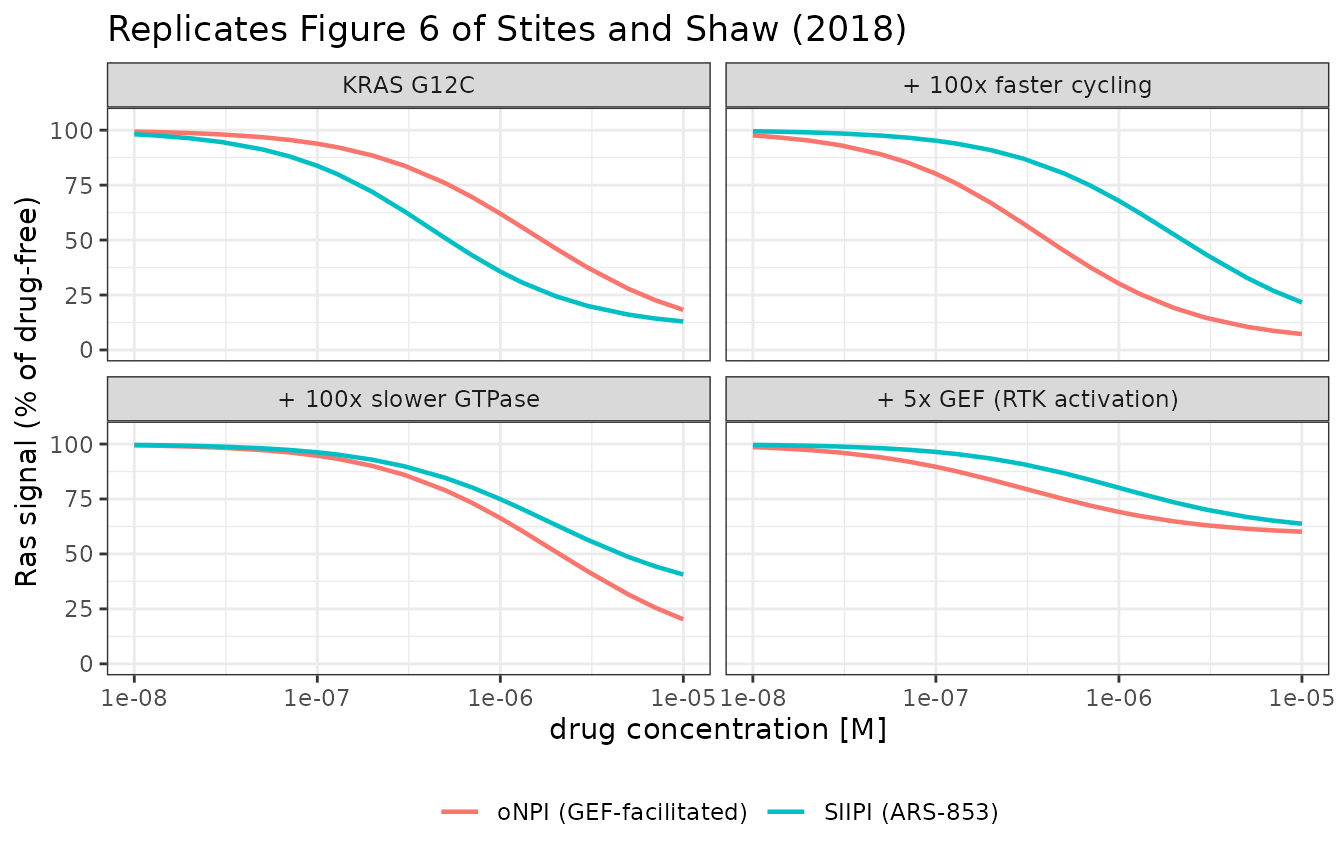

fig6_tab <- fig6 |>
  filter(dose == 1e-5) |>
  select(Case = case, Drug = drug, `Signal at 1e-5 M (%)` = signal) |>
  pivot_wider(names_from = Drug, values_from = `Signal at 1e-5 M (%)`)
kable(fig6_tab, digits = 1)

Case	SIIPI (ARS-853)	oNPI (GEF-facilitated)
KRAS G12C	12.9	18.2
+ 100x faster cycling	21.6	7.2
+ 100x slower GTPase	40.6	20.2
+ 5x GEF (RTK activation)	63.7	60.1


sii_v <- fig6_tab$`SIIPI (ARS-853)`
onp_v <- fig6_tab$`oNPI (GEF-facilitated)`

# 1. For plain KRAS G12C the SIIPI is the better inhibitor.
stopifnot(sii_v[1] < onp_v[1])
# 2. For a faster-cycling secondary mutation that ordering REVERSES: the SIIPI
#    gets worse while the oNPI gets BETTER than it was against plain G12C.
#    This is the paper's headline finding.
stopifnot(sii_v[2] > sii_v[1])
stopifnot(onp_v[2] < onp_v[1])
stopifnot(onp_v[2] < sii_v[2])
# 3. For the other two mechanisms both drugs lose potency, but the oNPI ends up
#    relatively better than the SIIPI in each case.
stopifnot(sii_v[3] > sii_v[1], onp_v[3] > onp_v[1], onp_v[3] < sii_v[3])
stopifnot(sii_v[4] > sii_v[1], onp_v[4] > onp_v[1], onp_v[4] < sii_v[4])

Comparison against the reported experimental potency

The paper validates itself against two published cell-culture measurements of ARS-853. There is no NCA here – the model has no pharmacokinetics, no dosing events and no residual error, so the appropriate comparison is the simulated concentration-response against the reported potency.

ars_signal <- pct_of_undosed(ars853$frac_eff_bound)
potency <- tibble::tibble(
  `Reported observation` = c(
    "IC50 of ARS-853, Lito 2016 (Science)",
    "IC50 of ARS-853, Patricelli 2016 (Cancer Discov)",
    "Ras signal reduction at 10 microM, Lito 2016"
  ),
  Reference = c("about 2.5 microM", "1 to 2 microM", "about 95%"),
  Simulated = c(
    sprintf("%.2f microM", approx(ars_signal, DOSES, xout = 50)$y * 1e6),
    sprintf("%.2f microM", approx(ars_signal, DOSES, xout = 50)$y * 1e6),
    sprintf("%.0f%%", 100 - ars_signal[DOSES == 1e-5])
  )
)
kable(potency)

Reported observation	Reference	Simulated
IC50 of ARS-853, Lito 2016 (Science)	about 2.5 microM	0.52 microM
IC50 of ARS-853, Patricelli 2016 (Cancer Discov)	1 to 2 microM	0.52 microM
Ras signal reduction at 10 microM, Lito 2016	about 95%	87%

The simulated half-maximal concentration sits just under 1 microM against a reported 1 to 2.5 microM, and the simulated reduction at 10 microM is about 87% against a reported 95%. The paper claims agreement at this level of precision and no better – its own wording is “roughly mirroring the experimental observations” and “comparable to the reductions in Ras signal found in our simulations” – and that is what the numbers show. The point the authors draw from it is structural rather than numerical: a covalent inhibitor has no Kd to tune, so the agreement cannot have come from fitting an affinity.

sim_ic50_um <- approx(ars_signal, DOSES, xout = 50)$y * 1e6
sim_red_10um <- 100 - ars_signal[DOSES == 1e-5]
# Within a factor of three of the reported potency range, and a reduction that
# is large but short of the reported 95%. Both bounds still fail loudly on a
# mis-transcribed on-rate, degradation rate or mutant fraction, each of which
# moves these by much more than the tolerance.
stopifnot(sim_ic50_um > 0.3, sim_ic50_um < 5)
stopifnot(sim_red_10um > 70, sim_red_10um < 95)

Assumptions and deviations

The published Figure 2c legend transposes the NPI and compound-12 SIIPI curves. This is the only disagreement between this reproduction and the paper, and it is a swap rather than a numerical difference. The deposited GenerateFigure2.m plots column 1 (NPI, on-rate 2e6) in red and column 2 (SIIPI compound 12, on-rate 0.12) in blue. Running the deposited model gives 74.1% of drug-free signal at 1e-5 M for the NPI and 96.2% for compound 12. The published panel shows its red “NPI” curve ending near 97% and its blue “SIIPI” curve ending near 74% – the two values, matched to the other series’ label.

Three things make this a labelling error in the figure rather than a transcription error here. The black ARS-853 curve and the grey no-turnover curve come out of the same code paths and match the published panel essentially exactly (13% and a 5% floor reached just past 1e-7 M). Compound 12 and ARS-853 differ only in kon_drug, so the code path that produces the verified black curve is the same one that produces 96.2% for compound 12. And the arithmetic is unambiguous: at the drug-free steady state the model holds 1.9e-14 M nucleotide-free G12C and 3.5e-8 M GDP-bound G12C, so the NPI capture-rate coefficient is 2e6 x 1.9e-14 = 3.9e-8 against 0.12 x 3.5e-8 = 4.2e-9 for compound 12 – an order of magnitude in the NPI’s favour, which is the ordering reported here.

The model is shipped as the deposited code specifies. The paper’s conclusions are unaffected: every argument in the text compares NPIs against ARS-853 (the only compound “consistently effective at inhibiting KRAS G12C lung cancer cells”), and the NPI is far weaker than ARS-853 under either reading.

The body text and Table 1 disagree on the NPI on-rate. Table 1 gives k on,NPI = 2e6 1/(M*s); the Results section says the NPI was modelled “with an on-rate similar to that for nucleotides (kon = 2e5 /Ms)”. The deposited code uses onrateNPI = 2e6 throughout, and the nucleotide association rates in that same code are 2.3e6 and 2.2e6 – so “similar to that for nucleotides” supports the table, not the text. 2e6 is used here.

Figure 1b is reproduced only in part. The deposited archive ships drivers for Figures 2 through 6. The G12V, G12D and F28L columns of Figure 1b require mutant scaling factors from Stites 2007 that are neither in this paper nor in the supplement, so they are omitted rather than guessed. The wild-type and G12C columns, and all of Figure 1c, are reproduced.

Steady state is reached by long integration rather than by iterated re-integration. The deposited driver repeatedly integrates a 10,000 s window until the state vector stops changing to within a 2-norm of 1e-15. Integrating once to 2e6 s reaches the same fixed point; the steady-state hold check above shows the last eight Ras half-lives move the answer by less than one part in 1e9.

GEF loading uses the nominal, not the free, inhibitor concentration. The deposited code computes the two GEF-loading maximal velocities once, from the scalar total NPI concentration passed into the driver (k(33) and k(34) are set from DrugConcNPI, not from the time-varying state y(13)). The model reproduces this by deriving vmaxd_npi and vmaxt_npi from the npi0 parameter. At the doses simulated the free and total NPI differ by at most a few percent, because total Ras is 4e-7 M against drug concentrations up to 1e-5 M.

One on-rate serves both drug classes. kon_drug maps to the deposited k(32) = kaDrug, which the ODE file uses for NPI binding and for both SIIPI binding reactions. Every published scenario gives only one of the two drugs, so the shared constant is always the on-rate of whichever compound is present. Do not set npi0 and siipi0 non-zero at once unless the two compounds genuinely share an on-rate.

No variability and no residual error. The paper fits nothing and estimates nothing: every constant is a literature biochemical rate or a parameter carried from the authors’ 2007 model. There is accordingly no IIV, no residual error model and no observation endpoint, and all assertions in this vignette are on deterministic quantities.

The no-turnover arm reduces the mutant pool rather than dosing a drug. RasG12C_inhibition_NT.m sets the degradation and both production rates to zero and passes the mutant total as 0.25 * 4e-7 - DrugConc, clamped at zero, with both free-drug concentrations at zero. That is reproduced literally above, which is why the no-turnover curve is identical for all three compounds – with the system closed, the on-rate no longer matters at steady state.

n_subjects and n_studies are zero. No humans or animals were studied. The population metadata records the simulated cellular composition instead: 50% of total Ras is KRAS and one KRAS allele is mutated, giving 25% KRAS G12C.