Competitive in vitro metabolism of benzo[a]pyrene and dibenzo[def,p]chrysene (Smith 2022)
Source:vignettes/articles/Smith_2022_pah_competitive_metabolism.Rmd
Smith_2022_pah_competitive_metabolism.RmdModel and source
- Citation: Smith JN, Gaither KA, Pande P. Competitive Metabolism of Polycyclic Aromatic Hydrocarbons (PAHs): An Assessment Using In Vitro Metabolism and Physiologically Based Pharmacokinetic (PBPK) Modeling. Int J Environ Res Public Health. 2022;19(14):8266. doi:10.3390/ijerph19148266. PMCID: PMC9323266. In vitro Michaelis-Menten-clearance parameters: Table 3; competitive-inhibition constants (Ki): Table 4; metabolism-rate equations: Eq. 2 (baseline, no inhibitor) and Eq. 4 (competitive inhibition raising the apparent Km1 of the saturable arm).
- Article: https://doi.org/10.3390/ijerph19148266
Smith and colleagues measured how two polycyclic aromatic
hydrocarbons (PAHs) – benzo[a]pyrene (BaP) and dibenzo[def,p]chrysene
(DBC) – compete for the cytochrome-P450 enzymes that metabolise them in
pooled human liver microsomes. Each parent disappears with saturable
kinetics characteristic of two dominant enzymes: a
high-affinity/low-capacity enzyme (a Michaelis-Menten
Vmax1/Km1 arm) and a
high-capacity/low-affinity enzyme that did not saturate over the tested
concentration range (a linear intrinsic-clearance Clint2
arm). This “Michaelis-Menten clearance” form (Eq. 2) was the best-fit
baseline model for both substrates by the Bayesian information criterion
(Table 2).
When the two PAHs are co-incubated, each raises the apparent
Km1 of the other’s saturable arm – classical competitive
inhibition (Eq. 4), again the BIC-best of the competitive forms tested.
The packaged model is the two coupled substrate-disappearance ODEs with
the per-mg-microsomal-protein kinetic constants of Tables 3-4.
This vignette validates the in vitro metabolism layer of the paper. The paper’s downstream whole-body PBPK interaction model inherits its physiology (compartment volumes, blood flows, partition coefficients, absorption rates) wholesale from the published DBC PBPK model (Pande 2022) and the BaP/DBC rodent PBPK models (Crowell 2011); those physiological parameters are not reported in this paper, so the PBPK layer is not reproduced here (see “Assumptions and deviations”).
Experimental system
| Field | Value |
|---|---|
| species | in vitro (pooled human liver microsomes) |
| n_subjects | 200 |
| n_studies | 1 |
| age_range | 19-78 years (3 donors 10-18 years) |
| sex_female_pct | 50 |
| disease_state | not applicable (pooled human liver microsomes) |
| notes | Pooled human liver microsomes (Sekisui Xenotech) contributed by 200 donors with an equal male:female ratio, predominantly 19-78 years (3 donors 10-18 years). Incubations (Methods 2.2): 2.0 mg/mL microsomal protein, 0.1 M phosphate buffer pH 7.4, 3 mM MgCl2, excess (1.5 mM) NADPH, 37 C. BaP 0.05-2.5 uM incubated 0-30 min; DBC 0.025-1 uM incubated 0-60 min. Competitive-inhibition assays held one PAH at a fixed substrate concentration (BaP 0.14-0.18 uM; DBC 0.17 uM) and co-incubated the other PAH across 0.1-10 uM. All kinetic parameters are per mg microsomal protein. Supermix-10 (a 10-PAH environmental mixture) was measured as an additional inhibitor (Ki 0.75 uM on BaP, 0.63 uM on DBC; Table 4) but the authors built no dynamical Supermix-10 model, so it is not encoded here. |
Pooled human liver microsomes (200 donors, equal male:female ratio) were incubated at 2.0 mg/mL microsomal protein in pH 7.4 phosphate buffer with excess NADPH at 37 C. Substrate disappearance was followed over 0-30 min (BaP) or 0-60 min (DBC), and initial rates were taken as the first-order slope of the concentration-time data. The model carries no between-donor random effects and no residual error: the publication reports parameter uncertainty as bootstrap confidence intervals on the point estimates, not as a hierarchical variance, so the packaged model is deterministic.
Source trace
Every ini() entry carries an in-file comment naming its
source location; the table below collects them for review.
| Quantity | Value | Source |
|---|---|---|
| d/dt(bap), d/dt(dbc) | n/a | Eq. 4 (competitive); Eq. 2 at zero inhibitor |
| rate = Vmax1S/(Km1(1+I/Ki)+S)+Clint2*S | n/a | Eq. 4 |
| Clint1 = Vmax1/Km1 | n/a | Methods 2.5 |
| BaP Vmax1 | 0.0063 nmol/min/mg | Table 3 (95% CI 0.0044-0.0083) |
| BaP Km1 | 0.088 uM | Table 3 (0.044-0.15) |
| BaP Clint2 | 0.0012 mL/min/mg | Table 3 (1.7e-7 to 0.0028) |
| DBC Vmax1 | 0.00090 nmol/min/mg | Table 3 (0.00044-0.0023) |
| DBC Km1 | 0.060 uM | Table 3 (0.014-0.22) |
| DBC Clint2 | 0.0017 mL/min/mg | Table 3 (6.5e-7 to 0.0028) |
| Ki, DBC inhibiting BaP | 0.44 uM | Table 4 (0.36-0.54) |
| Ki, BaP inhibiting DBC | 0.061 uM | Table 4 (0.041-0.12) |
| Microsomal protein | 2.0 mg/mL | Methods 2.2 |
| Clint1 (reported) | BaP 0.072, DBC 0.015 | Table 3 |
Units and dimensional analysis
The per-mg metabolism rate is in nmol/min/mg microsomal protein, the
concentrations in uM (= nmol/mL), and time in minutes. Multiplying the
per-mg rate by the microsomal protein concentration cmic
(mg/mL) turns it into a concentration rate:
| Symbol | Units | Note |
|---|---|---|
| bap, dbc | uM = nmol/mL | ODE states: substrate concentration |
| vmax_bap, vmax_dbc | nmol/min/mg | Michaelis-Menten Vmax1 per mg protein |
| km_bap, km_dbc | uM | Michaelis-Menten Km1 |
| clint2_bap, clint2_dbc | mL/min/mg | linear intrinsic clearance of the non-saturable arm |
| ki_dbc_bap, ki_bap_dbc | uM | competitive inhibition constants |
| rate_bap, rate_dbc | nmol/min/mg | per-mg disappearance rate (Eq. 4) |
| cmic | mg/mL | microsomal protein concentration |
| d/dt(bap) | uM/min | cmic * rate = (mg/mL)(nmol/min/mg) = nmol/mL/min |
Checking one term: clint2_bap * bap has units
(mL/min/mg)(nmol/mL) = nmol/min/mg, which matches the Vmax arm, and the
inhibition factor 1 + dbc/ki is a dimensionless ratio of
two uM quantities, so rate_bap is nmol/min/mg and
cmic * rate_bap is uM/min throughout.
Building a microsomal incubation
mod <- readModelDb("Smith_2022_pah_competitive_metabolism")

# One microsomal incubation as an rxode2 event table. The two substrates are
# "dosed" into their own ODE states at time 0 (a bolus into a concentration
# state sets that concentration, uM). Observation rows point at the ODE state
# `bap` (never at an algebraic observable such as rate_bap); rxSolve returns
# every state and derived column -- bap, dbc, rate_bap, rate_dbc -- at each
# observation time regardless of the row's compartment, so one obs row per time
# is enough and avoids duplicate output rows.
incubation <- function(times, id = 1L, bap0 = 0, dbc0 = 0) {
  tt <- sort(unique(c(0, times)))
  doses <- dplyr::bind_rows(
    if (bap0 > 0) tibble::tibble(id = id, time = 0, amt = bap0, evid = 1L, cmt = "bap"),
    if (dbc0 > 0) tibble::tibble(id = id, time = 0, amt = dbc0, evid = 1L, cmt = "dbc")
  )
  obs <- tibble::tibble(id = id, time = tt, amt = NA_real_, evid = 0L, cmt = "bap")
  dplyr::bind_rows(doses, obs) |>
    dplyr::arrange(id, time, dplyr::desc(evid))
}

# Initial per-mg disappearance rate at a given pair of starting concentrations,
# read from the model at time 0 (before measurable depletion). This is the
# quantity Figures 2-4 plot.
initial_rate <- function(bap0 = 0, dbc0 = 0) {
  s <- rxode2::rxSolve(mod, events = incubation(0, bap0 = bap0, dbc0 = dbc0),
                       returnType = "data.frame")
  s0 <- s[s$time == 0, ][1, ]
  c(rate_bap = s0$rate_bap, rate_dbc = s0$rate_dbc,
    clint1_bap = s0$clint1_bap, clint1_dbc = s0$clint1_dbc)
}
Structural checks
Two properties follow from the equations rather than from any fitted value, so they are exact and catch a sign error, a dropped term or a mis-typed constant immediately. The model carries no random effects, so every check below is deterministic.
r <- initial_rate(bap0 = 0.2, dbc0 = 0.2)

# 1. Clint1 = Vmax1/Km1, the first-order intrinsic clearance the paper reports
#    in Table 3 (BaP 0.072, DBC 0.015 mL/min/mg).
stopifnot(
  abs(r[["clint1_bap"]] - 0.0063 / 0.088) < 1e-9,
  abs(r[["clint1_dbc"]] - 0.00090 / 0.060) < 1e-9,
  abs(r[["clint1_bap"]] - 0.072) < 0.001,   # rounds to the Table 3 value
  abs(r[["clint1_dbc"]] - 0.015) < 1e-6     # exact to the Table 3 value
)

# 2. The model's initial-rate observable equals the Eq. 4 closed form. This pins
#    the observable/ODE wiring to the published equation.
eq4 <- function(S, I, vmax, km, clint2, ki) vmax * S / (km * (1 + I / ki) + S) + clint2 * S
stopifnot(
  abs(initial_rate(bap0 = 0.2, dbc0 = 0.5)[["rate_bap"]] -
        eq4(0.2, 0.5, 0.0063, 0.088, 0.0012, 0.44)) < 1e-9,
  abs(initial_rate(bap0 = 0.5, dbc0 = 0.17)[["rate_dbc"]] -
        eq4(0.17, 0.5, 0.00090, 0.060, 0.0017, 0.061)) < 1e-9
)

# 3. At low concentration and no inhibitor the saturable arm is first order, so
#    the total rate approaches (Clint1 + Clint2) * S (the approximation error is
#    O(S/Km1), so a very low S makes it exact to well under 0.1%).
low <- initial_rate(bap0 = 1e-6)[["rate_bap"]]
stopifnot(abs(low - (0.0063 / 0.088 + 0.0012) * 1e-6) / low < 1e-3)

tibble::tibble(
  Check = c("Clint1 BaP (mL/min/mg)", "Clint1 DBC (mL/min/mg)"),
  Model = round(c(r[["clint1_bap"]], r[["clint1_dbc"]]), 4),
  Published = c(0.072, 0.015)
) |>
knitr::kable(caption = "Structural check: Clint1 = Vmax1/Km1 against Table 3.")| Check | Model | Published |
|---|---|---|
| Clint1 BaP (mL/min/mg) | 0.0716 | 0.072 |
| Clint1 DBC (mL/min/mg) | 0.0150 | 0.015 |
Figure 2: substrate-saturation curves (no inhibitor)
Figure 2 of the paper plots the initial rate of disappearance against
substrate concentration for each PAH incubated alone. The model
reproduces it by reading rate_bap (or
rate_dbc) across a concentration grid with the other PAH
set to zero. The two-phase shape the paper describes – a rapid
first-order phase at low concentration giving way to a slower phase as
the high-affinity enzyme saturates – is the sum of the saturating
Vmax1 arm and the linear Clint2 arm.
bap_grid <- exp(seq(log(0.01), log(3.3), length.out = 40))
dbc_grid <- exp(seq(log(0.01), log(1.0), length.out = 40))

fig2 <- dplyr::bind_rows(
  tibble::tibble(PAH = "BaP", conc = bap_grid,
                 rate = vapply(bap_grid, function(s) initial_rate(bap0 = s)[["rate_bap"]], numeric(1))),
  tibble::tibble(PAH = "DBC", conc = dbc_grid,
                 rate = vapply(dbc_grid, function(s) initial_rate(dbc0 = s)[["rate_dbc"]], numeric(1)))
)

ggplot(fig2, aes(conc, rate)) +
  geom_line() +
  facet_wrap(~PAH, scales = "free") +
  labs(x = "Substrate concentration (uM)", y = "Rate (nmol/min/mg microsomal protein)",
       title = "Figure 2 - substrate-saturation curves",
       caption = "Replicates Figure 2 of Smith 2022 (no inhibitor).") +
  theme(legend.position = "none")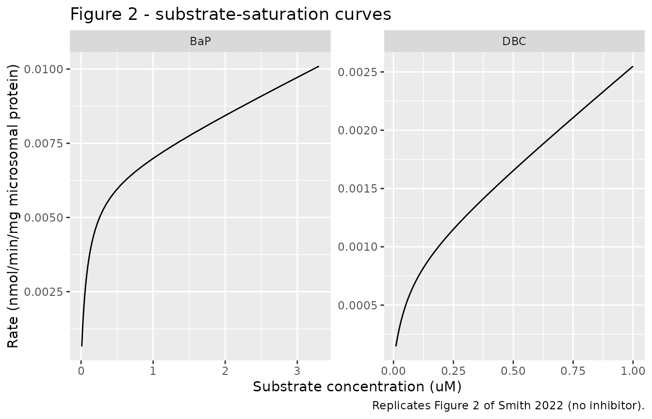
# BaP metabolism is 3-5x faster than DBC (Results 3.1). Compare the two at a
# shared 0.17 uM substrate concentration, where the paper quotes rates.
rate_bap_017 <- initial_rate(bap0 = 0.17)[["rate_bap"]]
rate_dbc_017 <- initial_rate(dbc0 = 0.17)[["rate_dbc"]]
fold <- rate_bap_017 / rate_dbc_017
stopifnot(fold > 3, fold < 5)   # paper: "DBC metabolism 3-5 times slower than BaP"

tibble::tibble(
  Quantity = c("BaP rate at 0.17 uM (nmol/min/mg)",
               "DBC rate at 0.17 uM (nmol/min/mg)",
               "BaP/DBC rate ratio"),
  Model = signif(c(rate_bap_017, rate_dbc_017, fold), 3),
  Published = c("-", "-", "3-5x (Results 3.1)")
) |>
knitr::kable(caption = "BaP metabolism is 3-5 times faster than DBC.")| Quantity | Model | Published |
|---|---|---|
| BaP rate at 0.17 uM (nmol/min/mg) | 0.004360 | - |
| DBC rate at 0.17 uM (nmol/min/mg) | 0.000954 | - |
| BaP/DBC rate ratio | 4.560000 | 3-5x (Results 3.1) |
Figures 3 and 4: competitive inhibition
Figure 3 holds BaP at a fixed low substrate concentration (0.14-0.18
uM) and co-incubates increasing DBC; Figure 4 holds DBC at 0.17 uM and
co-incubates increasing BaP. In each case the initial rate of the held
substrate falls as the competitor raises its apparent
Km1.
inh_grid <- exp(seq(log(0.05), log(10), length.out = 30))

fig34 <- dplyr::bind_rows(
  tibble::tibble(panel = "Fig 3: BaP (0.14 uM) inhibited by DBC",
                 inhibitor = inh_grid,
                 rate = vapply(inh_grid, function(i) initial_rate(bap0 = 0.14, dbc0 = i)[["rate_bap"]], numeric(1))),
  tibble::tibble(panel = "Fig 4: DBC (0.17 uM) inhibited by BaP",
                 inhibitor = inh_grid,
                 rate = vapply(inh_grid, function(i) initial_rate(bap0 = i, dbc0 = 0.17)[["rate_dbc"]], numeric(1)))
)

ggplot(fig34, aes(inhibitor, rate)) +
  geom_line() +
  facet_wrap(~panel, scales = "free") +
  scale_x_log10() +
  labs(x = "Inhibitor concentration (uM)", y = "Rate of held substrate (nmol/min/mg)",
       title = "Figures 3-4 - competitive inhibition of PAH metabolism",
       caption = "Replicates Figures 3A and 4A of Smith 2022.")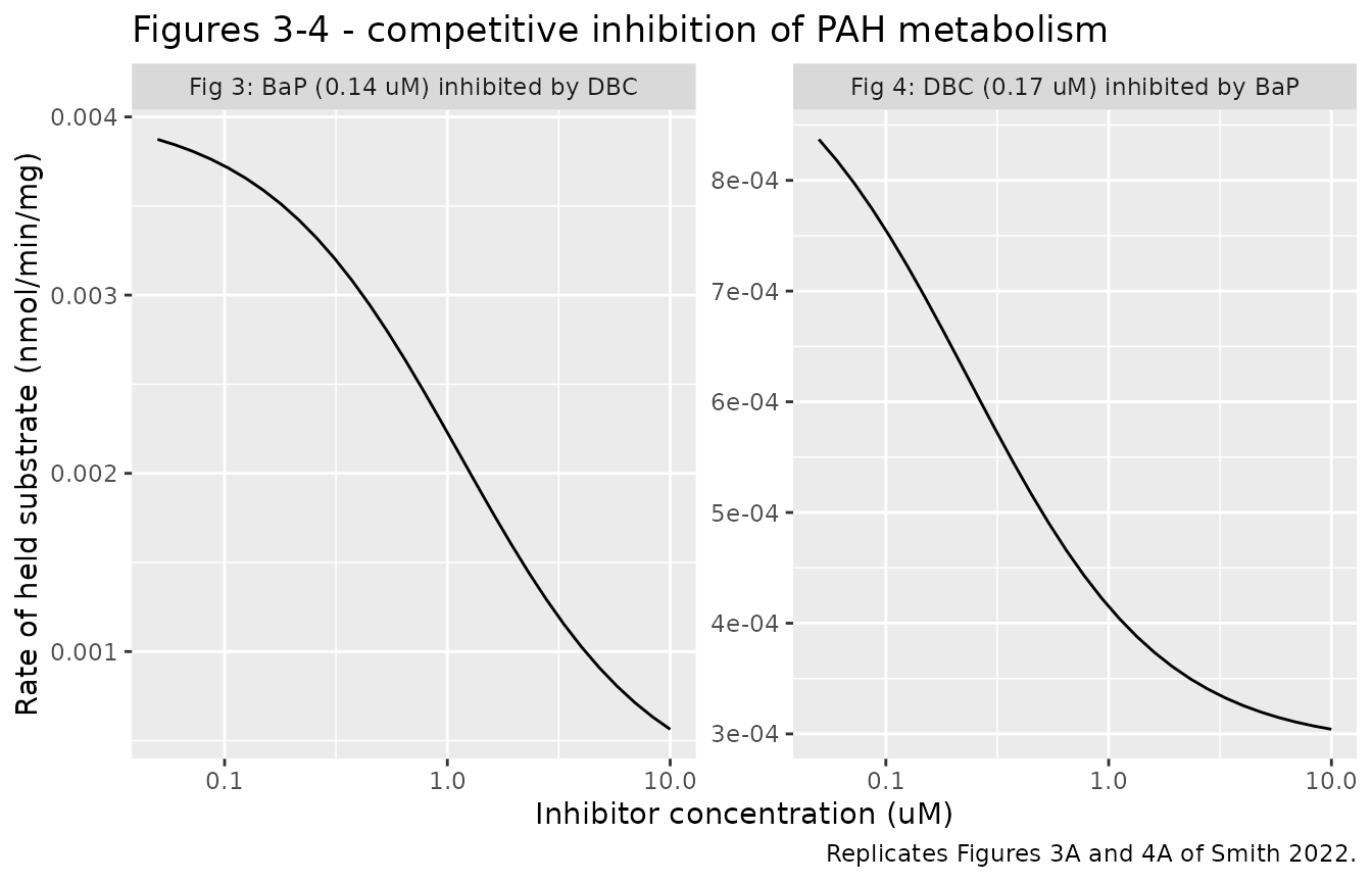
# The paper quotes specific observed inhibition percentages; the fitted Eq. 4
# model reproduces the direction and rough magnitude. These are observed values
# the model was fit to (not identities), so the bounds are set from the claims.
pct_inhib <- function(rate0, rate_inh) 100 * (1 - rate_inh / rate0)

# DBC (1 uM) inhibiting BaP metabolism at 0.14 uM BaP (Results: ">=48%").
bap_inh <- pct_inhib(initial_rate(bap0 = 0.14)[["rate_bap"]],
                     initial_rate(bap0 = 0.14, dbc0 = 1)[["rate_bap"]])
# BaP (1 uM) inhibiting DBC metabolism at 0.17 uM DBC (Results: "62%").
dbc_inh <- pct_inhib(initial_rate(dbc0 = 0.17)[["rate_dbc"]],
                     initial_rate(bap0 = 1, dbc0 = 0.17)[["rate_dbc"]])

# Monotonicity: more inhibitor always slows the held substrate.
fig3_rate <- fig34$rate[fig34$panel == "Fig 3: BaP (0.14 uM) inhibited by DBC"]
fig4_rate <- fig34$rate[fig34$panel == "Fig 4: DBC (0.17 uM) inhibited by BaP"]
stopifnot(
  all(diff(fig3_rate) < 0),
  all(diff(fig4_rate) < 0),
  bap_inh > 40,   # paper observed >=48% at 1 uM DBC
  dbc_inh > 50    # paper observed 62% at 1 uM BaP
)

tibble::tibble(
  Scenario = c("DBC 1 uM inhibiting BaP (0.14 uM)",
               "BaP 1 uM inhibiting DBC (0.17 uM)"),
  `Model % inhibition` = round(c(bap_inh, dbc_inh), 0),
  `Observed (paper)` = c(">=48%", "62%")
) |>
knitr::kable(caption = "Competitive-inhibition percentages quoted in the paper versus the fitted model.")| Scenario | Model % inhibition | Observed (paper) |
|---|---|---|
| DBC 1 uM inhibiting BaP (0.14 uM) | 45 | >=48% |
| BaP 1 uM inhibiting DBC (0.17 uM) | 57 | 62% |
BaP is the more potent inhibitor of the two: its Ki
against DBC metabolism (0.061 uM) is about sevenfold lower than DBC’s
Ki against BaP metabolism (0.44 uM).
Substrate depletion over the incubation (coupled ODEs)
The figures above read the initial rate; this check integrates the coupled ODEs over the full incubation window to confirm the dynamical system behaves. BaP and DBC are co-incubated, and the presence of each competitor slows the other’s disappearance relative to a single-substrate incubation.
grid <- seq(0, 60, by = 0.5)
# BaP alone vs BaP with DBC co-incubated.
bap_alone <- rxode2::rxSolve(mod, events = incubation(grid, id = 1L, bap0 = 1.0),
                             returnType = "data.frame")
bap_both  <- rxode2::rxSolve(mod, events = incubation(grid, id = 2L, bap0 = 1.0, dbc0 = 1.0),
                             returnType = "data.frame")

dep <- dplyr::bind_rows(
  tibble::tibble(time = bap_alone$time, bap = bap_alone$bap, series = "BaP alone"),
  tibble::tibble(time = bap_both$time,  bap = bap_both$bap,  series = "BaP + 1 uM DBC")
)

ggplot(dep, aes(time, bap, linetype = series)) +
  geom_line() +
  labs(x = "Time (min)", y = "BaP concentration (uM)", linetype = NULL,
       title = "Coupled competitive metabolism slows BaP disappearance",
       caption = "BaP depletion with and without co-incubated DBC.") +
  theme(legend.position = "bottom")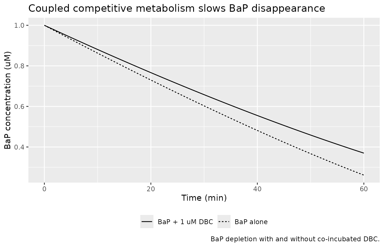
final_alone <- bap_alone$bap[bap_alone$time == 60]
final_both  <- bap_both$bap[bap_both$time == 60]
stopifnot(
  all(diff(bap_alone$bap) <= 1e-9),   # monotone non-increasing (substrate only disappears)
  all(bap_alone$bap >= -1e-9),        # concentrations stay non-negative
  final_both > final_alone            # co-incubated DBC slows BaP metabolism
)

tibble::tibble(
  Quantity = c("BaP remaining at 60 min, alone (uM)",
               "BaP remaining at 60 min, + 1 uM DBC (uM)"),
  Value = round(c(final_alone, final_both), 4)
) |>
knitr::kable(caption = "Competitive inhibition leaves more BaP at the end of the incubation.")| Quantity | Value |
|---|---|
| BaP remaining at 60 min, alone (uM) | 0.2613 |
| BaP remaining at 60 min, + 1 uM DBC (uM) | 0.3697 |
Assumptions and deviations
- Only the in vitro metabolism layer is packaged. The paper’s headline result is a whole-body PBPK interaction model that embeds these competitive metabolism equations. That model’s physiology – compartment volumes, blood flows, tissue/blood partition coefficients, absorption rates, and the liver volume used for the 30 mg-microsomal-protein-per-gram in vitro-to-in vivo scaling – is inherited wholesale from the published DBC human PBPK model (Pande 2022) and the BaP/DBC rodent PBPK models (Crowell 2011), neither of which reports those values in this paper. Reconstructing the PBPK layer requires those upstream sources and is left for a follow-up once they are obtained; substituting physiological constants from general knowledge would make the model unauditable.
- Supermix-10 is not encoded. The paper also measured inhibition constants for Supermix-10, a 10-PAH environmental mixture, on BaP (Ki 0.75 uM) and DBC (Ki 0.63 uM) metabolism (Table 4). The authors built no dynamical model for Supermix-10 – they note that doing so properly would require ten additional PBPK models – so it is carried only as a measured comparison in the population notes, not as a model state or parameter.
-
Deterministic, no residual error. Parameter
uncertainty is reported as bootstrap 95% confidence intervals on the
point estimates (Tables 3-4), not as a hierarchical between-donor
variance or a residual-error model, so the packaged model carries no
etaterms and no residual error. - The quoted inhibition percentages are observed, not identities. The paper’s “>=48%” (DBC on BaP) and “62%” (BaP on DBC) are measured inhibition at 1 uM competitor; the fitted Eq. 4 model reproduces the direction and rough magnitude (about 45% and 57% respectively) but is a fit to these data, not an exact reproduction of them.
-
Microsomal protein concentration is an incubation
condition.
cmicis fixed at the 2.0 mg/mL used in the assays (Methods 2.2); the per-mg kinetic constants are independent of it, so a user studying a different microsomal density can overridecmicwithout changing the fitted parameters. ```