Immune checkpoint inhibitor adverse events (Shulgin 2020)
Source:vignettes/articles/Shulgin_2020_ici_adverse_events_mbma.Rmd
Shulgin_2020_ici_adverse_events_mbma.RmdModel and source
Shulgin et al. pooled the published safety data of the anti-PD-1 antibodies nivolumab and pembrolizumab and the anti-CTLA-4 antibodies ipilimumab and tremelimumab, as monotherapy and in combination, and asked whether adverse-event (AE) rates depend on dose. To put different antibodies and dosing regimens on one axis, each cohort’s regimen was converted to a steady-state average serum concentration with a published population PK model and divided by the antibody’s in vitro IC50. Logit-transformed AE rates were then regressed on that normalized exposure.
- Article: https://doi.org/10.1080/2162402X.2020.1748982 (PMC7466858), Oncoimmunology. 2020;9(1):1748982.
- Supplement (Supplemental Methods and Supplemental Tables 1-5) on the publisher’s website; the fitted meta-regression coefficients are in Supplemental Tables 1-3.
The paper contributes four models, all study-level logit meta-regressions with no time axis:
| Model | Endpoint | Source |
|---|---|---|
Shulgin_2020_ici_trae34_mbma |
grade 3/4 treatment-related AE (trAE) | Supplemental Table 1, Model 4 (147 cohorts) |
Shulgin_2020_ici_gi_imae34_mbma |
grade 3/4 gastrointestinal immune-mediated AE (imAE) | Supplemental Table 1, Model 4 (62 cohorts) |
Shulgin_2020_ici_hepatic_imae34_mbma |
grade 3/4 hepatic imAE | Supplemental Table 1, Model 4 (62 cohorts) |
Shulgin_2020_ici_trae34_covariate_mbma |
grade 3/4 trAE with chemotherapy and line of therapy | Supplemental Table 3 (122 cohorts) |
mod_names <- c(
  trae = "Shulgin_2020_ici_trae34_mbma",
  gi = "Shulgin_2020_ici_gi_imae34_mbma",
  hepatic = "Shulgin_2020_ici_hepatic_imae34_mbma",
  trae_cov = "Shulgin_2020_ici_trae34_covariate_mbma"
)
mods <- lapply(mod_names, function(n) rxode2::rxode(readModelDb(n)))
coefs <- lapply(mods, function(m) stats::setNames(m$iniDf$est, m$iniDf$name))
Structure
“Model 4” of the paper (CTLA-4 inhibitor-driven, with PD-1 inhibitor-dependent modulation) was selected for all three endpoints:
where
is the normalized anti-CTLA-4 exposure (CAV / IC50_CTLA4)
and FactorPD1 (TRT_ANTIPD1) is 1 when the regimen contains
an anti-PD-1 antibody. Anti-PD-1 exposure has no effect, so anti-PD-1
monotherapy is predicted at
whatever its dose.
The covariate model adds chemotherapy given with an anti-PD-1 antibody () and a lower exposure slope for second-line-or-later therapy ():
with Line2+ formed as 1 - LINE_1L.
Population
The analysis pooled 153 treatment cohorts (21,305 patients) from 80 clinical trials published 2005-2018 and identified by a PRISMA search of PubMed-Medline, Citeline Trialtrove and ASCO / ESMO abstracts. Most cohorts were melanoma (58) or non-small cell lung cancer (37); renal cell, gastric, urothelial, small-cell lung, head and neck and other solid tumours make up the rest (Supplemental Table 5). Cohort median ages ranged 42-74 years (mean 60.6), and on average 61.2% of patients were male (Supplemental Table 4). Of 127 cohorts with a single line of therapy, 51 were first-line and 76 second-line or later; 27 cohorts received anti-PD-1 + anti-CTLA-4 combination therapy, and 16 received an immune checkpoint inhibitor with chemotherapy. Cancer type, the individual antibody within a target class, age, sex and PD-L1 positivity were screened and not retained (Supplemental Table 2).
The same information is available programmatically via each model’s
population metadata,
e.g. rxode2::rxode(readModelDb("Shulgin_2020_ici_trae34_mbma"))$population.
Source trace
| Equation / parameter | Value | Source location |
|---|---|---|
| Model 4 equation | n/a | Methods, “Statistical analysis”, Model 4 |
cnorm_ctla4 <- CAV / IC50_CTLA4 |
n/a | Supplemental Methods, “Pharmacokinetic models” |
trAE logit_ref
() |
-1.44 | Supplemental Table 1, trAE Model 4 row |
trAE e_cnorm_ctla4_logit
() |
0.0015 | Supplemental Table 1; main text Results |
trAE e_cnorm_ctla4_antipd1_logit
() |
0.011 | Supplemental Table 1 ( = 0.0124 in main text Results) |
GI logit_ref
|
-3.4 | Supplemental Table 1, GI Model 4 row |
GI e_cnorm_ctla4_logit
|
0.003 | Supplemental Table 1, GI Model 4 row |
GI e_cnorm_ctla4_antipd1_logit
|
0.01 | Supplemental Table 1, GI Model 4 row |
hepatic logit_ref
|
-3.6 | Supplemental Table 1, hepatic Model 4 row |
hepatic e_cnorm_ctla4_logit
|
0.002 | Supplemental Table 1, hepatic Model 4 row |
hepatic e_cnorm_ctla4_antipd1_logit
|
0.014 | Supplemental Table 1 prints 0.0014; see Errata |
covariate logit_ref
|
-1.53 | Supplemental Table 3, row 7 |
covariate e_cnorm_ctla4_logit
|
0.004 | Supplemental Table 3, row 7 |
covariate e_cnorm_ctla4_antipd1_logit
|
0.01 | Supplemental Table 3, row 7 |
covariate e_chemo_antipd1_logit
() |
1.1 | Supplemental Table 3, row 7 |
covariate e_cnorm_ctla4_line2_logit
() |
-0.003 | Supplemental Table 3, row 7 |
addSd_prob_* |
0.001 (fixed) | not from source; see Assumptions |
| PK parameters and IC50 values used below | see table | Supplemental Methods table |
Deriving the exposure input
The models do not take a dose. The input is the cohort’s steady-state
average anti-CTLA-4 concentration CAV (nM) and the
antibody’s IC50_CTLA4 (nM). The Supplemental Methods give
the two-compartment PK parameters and IC50 values the authors used and
say that concentrations were “averaged over time intervals corresponding
to between 3 and 4 delivered doses”. Below, each regimen is simulated
with those parameters, and PKNCA computes the average concentration over
the interval between the 3rd and 4th doses.
pk_par <- tibble::tribble(
  ~drug,           ~target,  ~ic50_printed, ~vc,  ~cl,    ~vp,  ~q,
  "nivolumab",     "PD-1",   1.04,          3.63, 0.0094, 2.78, 0.0320,
  "pembrolizumab", "PD-1",   0.62,          3.48, 0.0092, 4.06, 0.0331,
  "ipilimumab",    "CTLA-4", 13.3,          4.15, 0.0150, 3.11, 0.0411,
  "tremelimumab",  "CTLA-4", 0.65,          3.72, 0.0109, 3.31, 0.0172
)
pk_par |>
  dplyr::rename(
    Drug = drug, Target = target, "IC50 (nM)" = ic50_printed,
    "Vc (L)" = vc, "CL (L/h)" = cl, "Vp (L)" = vp, "Q (L/h)" = q
  ) |>
knitr::kable(caption = "Supplemental Methods table of Shulgin 2020.")| Drug | Target | IC50 (nM) | Vc (L) | CL (L/h) | Vp (L) | Q (L/h) |
|---|---|---|---|---|---|---|
| nivolumab | PD-1 | 1.04 | 3.63 | 0.0094 | 2.78 | 0.0320 |
| pembrolizumab | PD-1 | 0.62 | 3.48 | 0.0092 | 4.06 | 0.0331 |
| ipilimumab | CTLA-4 | 13.30 | 4.15 | 0.0150 | 3.11 | 0.0411 |
| tremelimumab | CTLA-4 | 0.65 | 3.72 | 0.0109 | 3.31 | 0.0172 |
pk_mod <- rxode2::rxode2({
  d / dt(central) <- -cl / vc * central - q / vc * central + q / vp * peripheral1
  d / dt(peripheral1) <- q / vc * central - q / vp * peripheral1
  Cc <- central / vc
})

# Regimens from Supplemental Table 5, with the maintainers' reading of where each
# one sits on the x-axis of main-text Figure 2a (grade 3/4 trAE panels).
regimens <- tibble::tribble(
  ~regimen,                 ~drug,           ~mgkg, ~tau_wk, ~fig2_position,
  "ipilimumab 1 mg/kg Q12W", "ipilimumab",    1,     12,      12,
  "ipilimumab 1 mg/kg Q6W",  "ipilimumab",    1,     6,       22,
  "ipilimumab 1 mg/kg Q3W",  "ipilimumab",    1,     3,       45,
  "ipilimumab 3 mg/kg Q3W",  "ipilimumab",    3,     3,       140,
  "ipilimumab 10 mg/kg Q3W", "ipilimumab",    10,    3,       430,
  "tremelimumab 15 mg/kg Q12W", "tremelimumab", 15, 12,       430,
  "tremelimumab 10 mg/kg Q4W",  "tremelimumab", 10, 4,        930,
  "nivolumab 3 mg/kg Q2W",   "nivolumab",     3,     2,       370,
  "nivolumab 10 mg/kg Q3W",  "nivolumab",     10,    3,       900,
  "pembrolizumab 2 mg/kg Q3W", "pembrolizumab", 2,   3,       310,
  "pembrolizumab 10 mg/kg Q2W", "pembrolizumab", 10, 2,       2400
) |>
  dplyr::left_join(pk_par, by = "drug") |>
  dplyr::mutate(id = dplyr::row_number(), tau = tau_wk * 168)

wt <- 70 # kg; see Assumptions
mw <- 148000 # g/mol, IgG; see Assumptions

sim_one <- function(r) {
  obs_times <- sort(unique(c(seq(0, 4 * r$tau, length.out = 801), 2 * r$tau, 3 * r$tau)))
  ev <- rxode2::et(amt = r$mgkg * wt, ii = r$tau, addl = 3, cmt = "central") |>
    rxode2::et(obs_times, cmt = "central")
  s <- rxode2::rxSolve(
    pk_mod,
    params = c(vc = r$vc, cl = r$cl, vp = r$vp, q = r$q),
    events = ev, returnType = "data.frame"
  )
  data.frame(id = r$id, regimen = r$regimen, time = s$time, Cc = s$Cc)
}
conc <- dplyr::bind_rows(lapply(split(regimens, regimens$id), sim_one))

dose_df <- dplyr::bind_rows(lapply(split(regimens, regimens$id), function(r) {
  data.frame(id = r$id, regimen = r$regimen, time = r$tau * 0:3, amt = r$mgkg * wt)
}))

conc_obj <- PKNCA::PKNCAconc(
  dplyr::filter(conc, !is.na(Cc)), Cc ~ time | regimen + id,
  concu = "mg/L", timeu = "h"
)
dose_obj <- PKNCA::PKNCAdose(dose_df, amt ~ time | regimen + id,
  doseu = "mg"
)
intervals <- regimens |>
  dplyr::transmute(regimen, id, start = 2 * tau, end = 3 * tau, cav = TRUE)
nca <- PKNCA::pk.nca(PKNCA::PKNCAdata(conc_obj, dose_obj, intervals = intervals))

cav <- as.data.frame(nca$result) |>
  dplyr::filter(PPTESTCD == "cav") |>
  dplyr::select(id, cav_mgL = PPORRES)

exposure <- regimens |>
  dplyr::left_join(cav, by = "id") |>
  dplyr::mutate(
    cav_nM = cav_mgL / mw * 1e6,
    cav_ss_nM = mgkg * wt / (cl * tau) / mw * 1e6,
    norm_printed = cav_nM / ic50_printed,
    ic50_used = ifelse(drug == "ipilimumab", 1.33, ic50_printed),
    norm_used = cav_nM / ic50_used
  )

exposure |>
  dplyr::select(regimen, cav_nM, cav_ss_nM, norm_printed, norm_used, fig2_position) |>
  dplyr::mutate(dplyr::across(where(is.numeric), ~ signif(.x, 3))) |>
  dplyr::rename(
    Regimen = regimen,
    "Cav doses 3-4 (nM)" = cav_nM,
    "Dose/(CL tau) (nM)" = cav_ss_nM,
    "Cav/IC50, printed IC50" = norm_printed,
    "Cav/IC50, ipilimumab 1.33 nM" = norm_used,
    "Figure 2 position" = fig2_position
  ) |>
knitr::kable(caption = "Normalized exposure by regimen at 70 kg.")| Regimen | Cav doses 3-4 (nM) | Dose/(CL tau) (nM) | Cav/IC50, printed IC50 | Cav/IC50, ipilimumab 1.33 nM | Figure 2 position |
|---|---|---|---|---|---|
| ipilimumab 1 mg/kg Q12W | 15.9 | 15.6 | 1.20 | 12.0 | 12 |
| ipilimumab 1 mg/kg Q6W | 31.5 | 31.3 | 2.37 | 23.7 | 22 |
| ipilimumab 1 mg/kg Q3W | 59.7 | 62.6 | 4.49 | 44.9 | 45 |
| ipilimumab 3 mg/kg Q3W | 179.0 | 188.0 | 13.50 | 135.0 | 140 |
| ipilimumab 10 mg/kg Q3W | 597.0 | 626.0 | 44.90 | 449.0 | 430 |
| tremelimumab 15 mg/kg Q12W | 328.0 | 323.0 | 504.00 | 504.0 | 430 |
| tremelimumab 10 mg/kg Q4W | 612.0 | 646.0 | 941.00 | 941.0 | 930 |
| nivolumab 3 mg/kg Q2W | 346.0 | 449.0 | 332.00 | 332.0 | 370 |
| nivolumab 10 mg/kg Q3W | 886.0 | 998.0 | 852.00 | 852.0 | 900 |
| pembrolizumab 2 mg/kg Q3W | 171.0 | 204.0 | 275.00 | 275.0 | 310 |
| pembrolizumab 10 mg/kg Q2W | 1080.0 | 1530.0 | 1750.00 | 1750.0 | 2400 |
The PKNCA average over the 3rd-4th dosing interval does not exceed
the closed-form steady-state value Dose / (CL * tau) beyond
trapezoidal error, because accumulation is not yet complete. For the
anti-CTLA-4 regimens it is within 5% of steady state. For the anti-PD-1
regimens, whose two- and three-week intervals are short relative to
their half-lives, it is 10-30% lower. With the printed IC50 values, both
tremelimumab regimens land close to their Figure 2 positions, and the
anti-PD-1 regimens land between the 3rd-4th-interval and steady-state
values. Every ipilimumab regimen, though, lands about
10-fold to the left of its Figure 2 position with the printed IC50 of
13.3 nM. With 1.33 nM, all five ipilimumab regimens land on their
plotted positions. The coefficients were fitted on the Figure 2 axis, so
use 1.33 nM for ipilimumab (see Errata).
ctla4 <- dplyr::filter(exposure, target == "CTLA-4")
ipi <- dplyr::filter(exposure, drug == "ipilimumab")
stopifnot(
  # The 3rd-4th interval average does not exceed the closed-form steady state
  # beyond trapezoidal error, and for the anti-CTLA-4 regimens it is within 6%.
  all(exposure$cav_nM < exposure$cav_ss_nM * 1.02),
  all(abs(ctla4$cav_nM / ctla4$cav_ss_nM - 1) < 0.06),
  # With ipilimumab normalized by 1.33 nM, every CTLA-4 regimen sits within 25%
  # of its Figure 2 position.
  all(abs(ctla4$norm_used / ctla4$fig2_position - 1) < 0.25),
  # With the printed 13.3 nM, every ipilimumab regimen is 7- to 13-fold low.
  all(ipi$fig2_position / ipi$norm_printed > 7),
  all(ipi$fig2_position / ipi$norm_printed < 13)
)
Replicating Figure 2
Figure 2 plots each endpoint against anti-PD-1 exposure (left panels; a flat line at ) and against anti-CTLA-4 exposure, for anti-CTLA-4 monotherapy and for combination with an anti-PD-1 antibody (right panels).
grid <- tidyr::expand_grid(
  CAV = exp(seq(log(10), log(1000), length.out = 200)),
  TRT_ANTIPD1 = c(0, 1)
) |>
  dplyr::mutate(id = dplyr::row_number(), time = 0, IC50_CTLA4 = 1)

solve_prob <- function(mod, data) {
  s <- rxode2::rxSolve(mod, data, returnType = "data.frame", keep = names(data))
  s[, grep("^prob_", names(s))[1]]
}
fig2 <- dplyr::bind_rows(lapply(c("trae", "gi", "hepatic"), function(k) {
  dplyr::mutate(grid, endpoint = k, p = solve_prob(mods[[k]], grid))
})) |>
  dplyr::mutate(
    endpoint = factor(endpoint,
      levels = c("trae", "gi", "hepatic"),
      labels = c("(a) total grade 3/4 trAE", "(b) GI imAE", "(c) hepatic imAE")
    ),
    regimen = ifelse(TRT_ANTIPD1 == 1, "anti-CTLA-4 + anti-PD-1", "anti-CTLA-4 monotherapy")
  )
#> Warning: There were 2 warnings in `dplyr::mutate()`.
#> The first warning was:
#> ℹ In argument: `p = solve_prob(mods[[k]], grid)`.
#> Caused by warning:
#> ! 'keep' contains id, time
#> which are output when needed, ignoring these items
#> ℹ Run `dplyr::last_dplyr_warnings()` to see the 1 remaining warning.
#> There were 2 warnings in `dplyr::mutate()`.
#> The first warning was:
#> ℹ In argument: `p = solve_prob(mods[[k]], grid)`.
#> Caused by warning:
#> ! 'keep' contains id, time
#> which are output when needed, ignoring these items
#> ℹ Run `dplyr::last_dplyr_warnings()` to see the 1 remaining warning.
#> There were 2 warnings in `dplyr::mutate()`.
#> The first warning was:
#> ℹ In argument: `p = solve_prob(mods[[k]], grid)`.
#> Caused by warning:
#> ! 'keep' contains id, time
#> which are output when needed, ignoring these items
#> ℹ Run `dplyr::last_dplyr_warnings()` to see the 1 remaining warning.

ggplot(fig2, aes(CAV, 100 * p, colour = regimen)) +
  geom_line(linewidth = 1) +
  scale_x_log10() +
  facet_wrap(~endpoint, ncol = 1, scales = "free_y") +
  coord_cartesian(ylim = c(0, NA)) +
  labs(
    x = "CTLA-4 ICI normalized exposure (Cav / IC50)",
    y = "Grade 3/4 AEs, %", colour = NULL
  ) +
  theme_bw() +
  theme(legend.position = "bottom")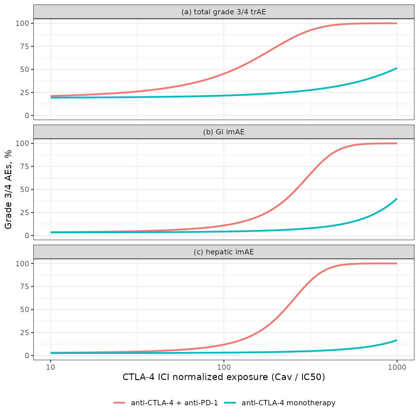
Replicates the right-hand panels of Figure 2 of Shulgin 2020 (model curves only; the cohort data points are not published in tabular form).
p_at <- function(k, cnorm, pd1) {
  d <- data.frame(id = 1, time = 0, CAV = cnorm, IC50_CTLA4 = 1, TRT_ANTIPD1 = pd1)
  solve_prob(mods[[k]], d)
}
# Maintainers' readings of the Figure 2a model curves: about 51% for monotherapy
# at a normalized exposure of 950, and about 57% for the combination at 140;
# PD-1 monotherapy (left panel) sits at about 19%.
stopifnot(
  abs(100 * p_at("trae", 950, 0) - 51) < 3,
  abs(100 * p_at("trae", 140, 1) - 57) < 3,
  abs(100 * p_at("trae", 0, 1) - 19) < 1.5
)
#> Warning: 'keep' contains id, time
#> which are output when needed, ignoring these items
#> Warning: 'keep' contains id, time
#> which are output when needed, ignoring these items
#> Warning: 'keep' contains id, time
#> which are output when needed, ignoring these items
# Main text Results: the CTLA-4 slope rises from 0.0015 to 0.0124 with an
# anti-PD-1 antibody; the table's beta1 + beta3 reproduces this within rounding.
stopifnot(abs(coefs$trae[["e_cnorm_ctla4_logit"]] +
  coefs$trae[["e_cnorm_ctla4_antipd1_logit"]] - 0.0124) < 0.0006)
Replicating Figure 3
Figure 3 uses the covariate model to predict grade 3/4 trAE rates for anti-PD-1 with and without chemotherapy (a), anti-CTLA-4 monotherapy by line of therapy (b), and the anti-CTLA-4 + anti-PD-1 combination with and without chemotherapy by line of therapy (c), including the triple combination that no trial had tested.
scen <- dplyr::bind_rows(
  # Panel (a): the x-axis is anti-PD-1 exposure, which is not a model input; the
  # anti-CTLA-4 input is 0 throughout.
  tidyr::expand_grid(panel = "(a) anti-PD-1", x = c(10, 1000), CAV = 0,
    TRT_ANTIPD1 = 1, CONMED_CHEMO = c(0, 1), LINE_1L = 1),
  tidyr::expand_grid(panel = "(b) anti-CTLA-4 monotherapy",
    CAV = exp(seq(log(10), log(1000), length.out = 100)), TRT_ANTIPD1 = 0,
    CONMED_CHEMO = 0, LINE_1L = c(0, 1)),
  tidyr::expand_grid(panel = "(c) anti-CTLA-4 + anti-PD-1",
    CAV = exp(seq(log(10), log(200), length.out = 100)), TRT_ANTIPD1 = 1,
    CONMED_CHEMO = c(0, 1), LINE_1L = c(0, 1))
) |>
  dplyr::mutate(
    id = dplyr::row_number(), time = 0, IC50_CTLA4 = 1,
    x = dplyr::coalesce(x, CAV)
  )
scen$p <- solve_prob(mods$trae_cov, scen)
#> Warning: 'keep' contains id, time
#> which are output when needed, ignoring these items
#> Warning: multi-subject simulation without without 'omega'
scen <- scen |>
  dplyr::mutate(scenario = paste0(
    ifelse(LINE_1L == 1, "first line", "second line or later"),
    ifelse(CONMED_CHEMO == 1, " + chemotherapy", "")
  ))

ggplot(scen, aes(x, 100 * p, colour = scenario)) +
  geom_line(linewidth = 1) +
  scale_x_log10() +
  facet_wrap(~panel, ncol = 2, scales = "free_x") +
  coord_cartesian(ylim = c(0, 100)) +
  labs(x = "Normalized exposure", y = "Grade 3/4 AEs, %", colour = NULL) +
  theme_bw() +
  theme(legend.position = "bottom")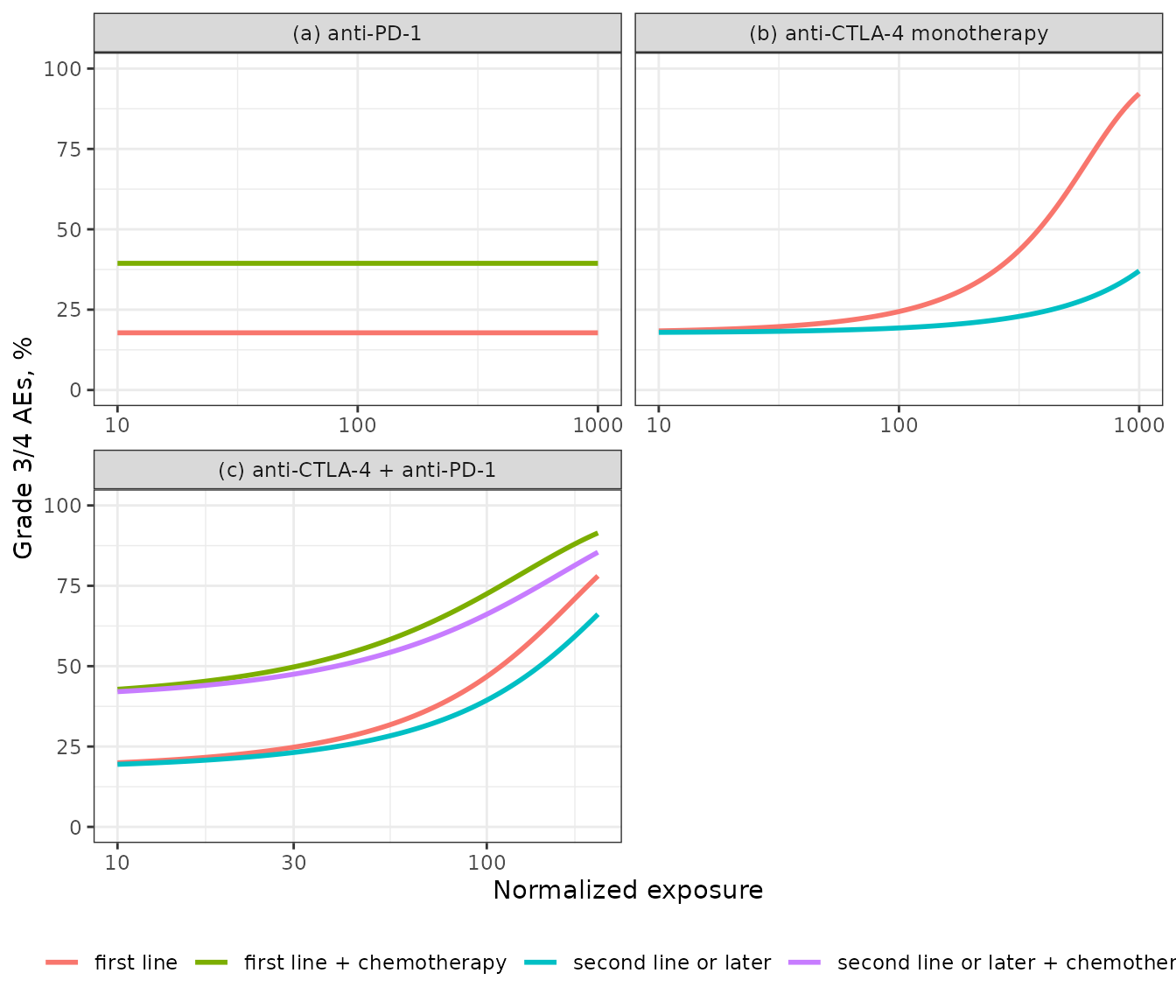
Replicates Figure 3 of Shulgin 2020 (typical-value curves only). In
panel (a) the x-axis is anti-PD-1 exposure, which has no effect; the
flat lines are computed at CAV = 0.
pd1 <- data.frame(
  id = 1:2, time = 0, CAV = 0, IC50_CTLA4 = 1, TRT_ANTIPD1 = 1,
  CONMED_CHEMO = c(0, 1), LINE_1L = 1
)
p_pd1 <- 100 * solve_prob(mods$trae_cov, pd1)
#> Warning: 'keep' contains id, time
#> which are output when needed, ignoring these items
#> Warning: multi-subject simulation without without 'omega'
knitr::kable(
  data.frame(
    Regimen = c("anti-PD-1 monotherapy", "anti-PD-1 + chemotherapy"),
    "Model (%)" = signif(p_pd1, 3),
    "Main text Results (%)" = c(17.7, 39.0),
    check.names = FALSE
  ),
  caption = "Grade 3/4 trAE rate: covariate model vs. the rates quoted in the main text."
)| Regimen | Model (%) | Main text Results (%) |
|---|---|---|
| anti-PD-1 monotherapy | 17.8 | 17.7 |
| anti-PD-1 + chemotherapy | 39.4 | 39.0 |
# The paper quotes 17.7% and 39.0%; the model's rounded coefficients give
# 17.8% and 39.4%.
stopifnot(abs(p_pd1[1] - 17.7) < 0.5, abs(p_pd1[2] - 39.0) < 0.8)

# Figure 3c, maintainers' readings: first-line combination about 80% at a
# normalized exposure of 200; triple combination about 42% at 10.
tri <- data.frame(
  id = 1:2, time = 0, CAV = c(200, 10), IC50_CTLA4 = 1, TRT_ANTIPD1 = 1,
  CONMED_CHEMO = c(0, 1), LINE_1L = 1
)
p_tri <- 100 * solve_prob(mods$trae_cov, tri)
#> Warning: 'keep' contains id, time
#> which are output when needed, ignoring these items
#> Warning: multi-subject simulation without without 'omega'
stopifnot(abs(p_tri[1] - 80) < 4, abs(p_tri[2] - 42) < 3)
Applying the model to a regimen
Combining the exposure derivation with the models gives predicted rates for specific regimens. Nivolumab 1 mg/kg + ipilimumab 3 mg/kg Q3W, the combination approved in melanoma, has a normalized ipilimumab exposure of about 135. Combination rows are shown only for the ipilimumab doses that combination cohorts actually received (1 and 3 mg/kg); the steep combination slope reaches 100% soon after the highest studied combination exposure, so predictions beyond it are extrapolation.
apply_df <- exposure |>
  dplyr::filter(target == "CTLA-4") |>
  dplyr::transmute(regimen, drug, mgkg, CAV = cav_nM, IC50_CTLA4 = ic50_used) |>
  tidyr::expand_grid(TRT_ANTIPD1 = c(0, 1)) |>
  # Combination cohorts in the analysis used ipilimumab 1 or 3 mg/kg only
  # (Supplemental Table 5); do not extrapolate the combination slope beyond them.
  dplyr::filter(TRT_ANTIPD1 == 0 | (drug == "ipilimumab" & mgkg <= 3)) |>
  dplyr::mutate(id = dplyr::row_number(), time = 0)
apply_df$trae <- solve_prob(mods$trae, apply_df)
#> Warning: 'keep' contains id, time
#> which are output when needed, ignoring these items
#> Warning: multi-subject simulation without without 'omega'
apply_df$gi <- solve_prob(mods$gi, apply_df)
#> Warning: 'keep' contains id, time
#> which are output when needed, ignoring these items
#> Warning: multi-subject simulation without without 'omega'
apply_df$hepatic <- solve_prob(mods$hepatic, apply_df)
#> Warning: 'keep' contains id, time
#> which are output when needed, ignoring these items
#> Warning: multi-subject simulation without without 'omega'
apply_df |>
  dplyr::mutate(
    with = ifelse(TRT_ANTIPD1 == 1, "+ anti-PD-1", "monotherapy"),
    dplyr::across(c(trae, gi, hepatic), ~ round(100 * .x, 1))
  ) |>
  dplyr::select(regimen, with, trae, gi, hepatic) |>
  dplyr::rename(
    "Anti-CTLA-4 regimen" = regimen, Setting = with,
    "Grade 3/4 trAE (%)" = trae, "Grade 3/4 GI imAE (%)" = gi,
    "Grade 3/4 hepatic imAE (%)" = hepatic
  ) |>
knitr::kable(caption = "Predicted cohort-level grade 3/4 AE rates (Model 4).")| Anti-CTLA-4 regimen | Setting | Grade 3/4 trAE (%) | Grade 3/4 GI imAE (%) | Grade 3/4 hepatic imAE (%) |
|---|---|---|---|---|
| ipilimumab 1 mg/kg Q12W | monotherapy | 19.4 | 3.3 | 2.7 |
| ipilimumab 1 mg/kg Q12W | + anti-PD-1 | 21.6 | 3.8 | 3.2 |
| ipilimumab 1 mg/kg Q6W | monotherapy | 19.7 | 3.5 | 2.8 |
| ipilimumab 1 mg/kg Q6W | + anti-PD-1 | 24.2 | 4.3 | 3.8 |
| ipilimumab 1 mg/kg Q3W | monotherapy | 20.2 | 3.7 | 2.9 |
| ipilimumab 1 mg/kg Q3W | + anti-PD-1 | 29.3 | 5.6 | 5.3 |
| ipilimumab 3 mg/kg Q3W | monotherapy | 22.5 | 4.8 | 3.5 |
| ipilimumab 3 mg/kg Q3W | + anti-PD-1 | 56.0 | 16.1 | 19.1 |
| ipilimumab 10 mg/kg Q3W | monotherapy | 31.7 | 11.4 | 6.3 |
| tremelimumab 15 mg/kg Q12W | monotherapy | 33.5 | 13.1 | 7.0 |
| tremelimumab 10 mg/kg Q4W | monotherapy | 49.3 | 36.0 | 15.2 |
Assumptions and deviations
-
Study-level model. All four models predict the
expected AE proportion of a trial cohort; they are not
individual-patient risk models. There is no time axis and no dose event:
exposure enters as the covariate columns
CAVandIC50_CTLA4. -
No residual or between-study variance. The paper
fits random-effects meta-regressions with metafor but does not report
the between-study variance. Each model carries a placeholder additive
residual
addSd_prob_* = fixed(0.001)so rxode2 has an error model; it is not a published quantity. UsezeroRe(), or read theprob_*column, for typical-value predictions. - Exposure derivation. The paper gives neither the body weight used for mg/kg doses nor the molecular weight used to convert mg/L to nM. This vignette uses 70 kg (the paper equates 200 mg pembrolizumab with 2.5 mg/kg at 70-75 kg) and 148 kDa. These values put the anti-PD-1 and tremelimumab regimens close to their Figure 2 positions. The averaging interval is read as the dosing interval between the 3rd and 4th doses.
- Choice of the covariate model. Supplemental Table 3 lists ten candidate covariate models and does not flag the selected one. Row 7 is shipped: it is the model with exactly the “two additional covariates” named in the main text, and the only Table 3 row that reproduces both quoted rates (17.7% and 39.0%) and the Figure 3 curves. The main text’s slope pair “0.0004 to 0.0034” for line of therapy comes from the single-covariate model in Supplemental Table 2 ( = 0.0034, = -0.003), not from this row. With row 7’s rounded coefficients (0.004, -0.003), the second-line-or-later monotherapy slope is 0.001 per unit, which puts the Figure 3b second-line curve above the one printed there.
-
Line of therapy. The source covariate
Line2+is encoded through the canonicalLINE_1Las1 - LINE_1L. Cohorts that mixed lines of therapy were excluded from the covariate analysis, so the model is defined only forLINE_1Lequal to 0 or 1. - Hepatic imAE curve. With the printed intercept of -3.6, the model reproduces the flat anti-PD-1 line of Figure 2c (about 3%). The anti-CTLA-4 panel of Figure 2c, however, starts at about 1.6% and reaches about 7% for monotherapy at a normalized exposure of 950, which corresponds to an intercept near -4.1. The printed table values are used; the hepatic model will predict higher rates than that panel shows.
Errata
- Ipilimumab IC50. The Supplemental Methods table prints an ipilimumab IC50 of 13.3 nM. On the exposure axis of Figure 2, which is the axis the coefficients were fitted on, all five ipilimumab regimens sit 10-fold higher than 13.3 nM gives, while tremelimumab and both anti-PD-1 antibodies sit where their printed values put them (see “Deriving the exposure input”). The value consistent with the fitted models is 1.33 nM, and the model files document 1.33 nM as the value to supply for ipilimumab. With 13.3 nM, predicted rates for ipilimumab regimens would be too low; for the nivolumab 1 mg/kg + ipilimumab 3 mg/kg combination the trAE prediction would fall from about 56% to about 22%.
- Hepatic imAE . Supplemental Table 1 prints = 0.0014 with SE 0.0021 and p < 0.001 for the hepatic Model 4 row. These three numbers cannot all hold (0.0014 is 0.67 SE, p about 0.5). The value 0.014 gives z = 6.7, consistent with the printed p-value; it matches the 0.014 in the neighbouring hepatic Model 3 row and the steep combination curve of Figure 2c. The model uses 0.014.
- Checked on 2026-09-27: no erratum or correction for this article was found.