Bispecific antibody TMDD: full model, QE approximation and optimal dosing (Schropp 2019)
Source:vignettes/articles/Schropp_2019_bsab_tmdd.Rmd
Schropp_2019_bsab_tmdd.RmdModel and source
- Article: https://doi.org/10.1002/psp4.12369 (CPT Pharmacometrics Syst Pharmacol. 2019;8(3):177-187, PMC6430159)
- Supplement: S1-S10, published with the open-access article (PMC6430159). S4/S6 are the authors’ MONOLIX/NONMEM code for the full model, S3/S5 for the quasi-equilibrium (QE) approximation with non-constant total receptors, and S8/S10 (with S7/S9 as the alternative representation) for the QE approximation with constant total receptors.
A bispecific antibody (BsAb) binds two different targets, so it can form two binary complexes and one ternary complex. The ternary complex – the “trimer” – is the species that physically bridges the two cells and therefore drives the pharmacodynamic effect. Schropp et al. write down a general target-mediated drug disposition (TMDD) model for this class, derive a quasi-equilibrium approximation that cuts the parameter count from 19 to 14 and then to 10, and use the reduced model to derive an optimal dosing strategy.
The paper’s central and counter-intuitive result is that more drug is not better. Because the trimer needs one free copy of each target, saturating both targets with binary complexes starves the cross-linking reaction, so the trimer concentration is a bell-shaped function of total drug and vanishes in the high-dose limit. Raising the dose therefore delays trimer build-up.
This is a theoretical / methodological paper: there is no clinical or preclinical dataset, no drug and no covariates. It contributes three models:
mods <- c(
  "Schropp_2019_bsab_tmdd_full",
  "Schropp_2019_bsab_tmdd_qe",
  "Schropp_2019_bsab_tmdd_qeconst"
)
full <- rxode2::rxode2(readModelDb(mods[1]))
qe <- rxode2::rxode2(readModelDb(mods[2]))
qeconst <- rxode2::rxode2(readModelDb(mods[3]))
#> ℹ parameter labels from comments will be replaced by 'label()'

tibble::tibble(
  Model = mods,
  `Paper equations` = c("Eqs 1-9", "Eqs 14-22, 24 + Table 1", "Eqs 15, 17, 23-30"),
  Parameters = c(19L, 14L, 10L),
  `ODE states` = c(length(full$state), length(qe$state), length(qeconst$state))
) |>
knitr::kable()| Model | Paper equations | Parameters | ODE states |
|---|---|---|---|
| Schropp_2019_bsab_tmdd_full | Eqs 1-9 | 19 | 8 |
| Schropp_2019_bsab_tmdd_qe | Eqs 14-22, 24 + Table 1 | 14 | 6 |
| Schropp_2019_bsab_tmdd_qeconst | Eqs 15, 17, 23-30 | 10 | 3 |
Population
There is no population. The paper fits no data: its parameter values
are a generic set “roughly based on literature reported values”
(Methods, Parameter setting for simulations; Table 2, left-hand
block), and its only subject-level exercise is a simulation-estimation
study in which 30 simulated individuals are generated with the
full model and refitted with the constant-total-receptor approximation.
Every ini() value is therefore wrapped in
fixed(), exactly as every $THETA in the
authors’ own NONMEM streams carries FIX.
pop <- readModelDb(mods[1])() |> environment() |> (\(e) e$population)()
tibble::tibble(Field = names(pop), Value = vapply(pop, \(x) paste(as.character(x), collapse = " "), "")) |>
knitr::kable()| Value |
|---|
Units and the dose conversion
Time is days, concentrations are nM, doses are nmol. The paper works in mg and states a conversion factor of 1 mg = 6.7 nmol (Methods, Parameter setting for simulations). That factor is load-bearing for every mg-denominated result below, so it is checked against two independent numbers the paper prints itself.
MG_TO_NMOL <- 6.7 # Methods, "Parameter setting for simulations"
VC <- 3 # Table 2, V = 3 L

tibble::tibble(
  Check = c(
    "S5/S9 NONMEM dataset comment: 50 mg i.v. bolus of Figure 3",
    "Eq 39 worked example: dose achieving Ctot(0) = 100 nM in 3 L"
  ),
  `Paper value` = c("335 nmol", "44.8 mg"),
  Reproduced = c(
    sprintf("%.1f nmol", 50 * MG_TO_NMOL),
    sprintf("%.1f mg", 100 * VC / MG_TO_NMOL)
  )
) |>
knitr::kable()| Check | Paper value | Reproduced |
|---|---|---|
| S5/S9 NONMEM dataset comment: 50 mg i.v. bolus of Figure 3 | 335 nmol | 335.0 nmol |
| Eq 39 worked example: dose achieving Ctot(0) = 100 nM in 3 L | 44.8 mg | 44.8 mg |
Both reproduce exactly, so the conversion factor is confirmed from inside the paper rather than assumed.
Source trace
tibble::tribble(
  ~Quantity, ~`Source location`,
  "d/dt AD, C, R_A, R_B, RC_A, RC_B, RC_AB, AP (full model)", "Eqs 1-8; authors' NONMEM DADT(1)-DADT(8) in S6",
  "Initial conditions R_X(0) = ksynX/kdegX, all else 0", "Eq 9; A_0(1)-A_0(8) in S6",
  "Total drug / total receptor definitions", "Eqs 11-13",
  "K_DZ = k_offZ / k_onZ", "Eq 14a",
  "Microscopic reversibility K_D1*K_D3 = K_D2*K_D4; K_D3 = alpha*K_D2, K_D4 = alpha*K_D1", "Eq 14b and following text",
  "QE matrix form d/dt(C, R_A, R_B) = M * g", "Eqs 15-19",
  "Matrix entries m_ij and determinant", "Table 1; written out in FORTRAN in S5/S9/S10",
  "Algebraic complexes RC_A, RC_B, RC_AB", "Eqs 20-22",
  "Constant-total-receptor reduction k_degX = k_intX = k_intAB = k_int", "Eq 23; assignments in S9/S10 $PK",
  "Single-ODE form, quadratic for R_B, explicit R_A", "Eqs 25-30; S10 $DES",
  "Trimer vanishes as C grows without bound", "Eq 35",
  "Optimal working range min(RtotA,RtotB) <= Ctot <= max(RtotA,RtotB)", "Eq 36",
  "Optimal initial dose, re-dosing time, subsequent doses", "Eqs 39, 40, 41",
  "Dummy i.v. input compartment", "Eq 42; TDUR = 0.0001 day in S5/S9/S10",
  "V, ka, F, kel, k12, k21, kon1-2, koff1-2, ksynA/B, kdegA/B, kintA/B/AB", "Table 2, left-hand 'Simulation' block",
  "kon3 = kon2, kon4 = kon1, koff3 = koff2, koff4 = koff1", "Table 2 footnote",
  "True and fitted kel, K_D1, K_D2, alpha, R0A, R0B, kint, V, omegas, b1-b3", "Table 2, right-hand 'Simulation-estimation' block",
  "1 mg = 6.7 nmol", "Methods, 'Parameter setting for simulations'",
  "LLOQ 0.01 nM", "Methods, 'Parameter setting for simulations'"
) |>
knitr::kable()| Quantity | Source location |
|---|---|
| d/dt AD, C, R_A, R_B, RC_A, RC_B, RC_AB, AP (full model) | Eqs 1-8; authors’ NONMEM DADT(1)-DADT(8) in S6 |
| Initial conditions R_X(0) = ksynX/kdegX, all else 0 | Eq 9; A_0(1)-A_0(8) in S6 |
| Total drug / total receptor definitions | Eqs 11-13 |
| K_DZ = k_offZ / k_onZ | Eq 14a |
| Microscopic reversibility K_D1K_D3 = K_D2K_D4; K_D3 = alphaK_D2, K_D4 = alphaK_D1 | Eq 14b and following text |
| QE matrix form d/dt(C, R_A, R_B) = M * g | Eqs 15-19 |
| Matrix entries m_ij and determinant | Table 1; written out in FORTRAN in S5/S9/S10 |
| Algebraic complexes RC_A, RC_B, RC_AB | Eqs 20-22 |
| Constant-total-receptor reduction k_degX = k_intX = k_intAB = k_int | Eq 23; assignments in S9/S10 $PK |
| Single-ODE form, quadratic for R_B, explicit R_A | Eqs 25-30; S10 $DES |
| Trimer vanishes as C grows without bound | Eq 35 |
| Optimal working range min(RtotA,RtotB) <= Ctot <= max(RtotA,RtotB) | Eq 36 |
| Optimal initial dose, re-dosing time, subsequent doses | Eqs 39, 40, 41 |
| Dummy i.v. input compartment | Eq 42; TDUR = 0.0001 day in S5/S9/S10 |
| V, ka, F, kel, k12, k21, kon1-2, koff1-2, ksynA/B, kdegA/B, kintA/B/AB | Table 2, left-hand ‘Simulation’ block |
| kon3 = kon2, kon4 = kon1, koff3 = koff2, koff4 = koff1 | Table 2 footnote |
| True and fitted kel, K_D1, K_D2, alpha, R0A, R0B, kint, V, omegas, b1-b3 | Table 2, right-hand ‘Simulation-estimation’ block |
| 1 mg = 6.7 nmol | Methods, ‘Parameter setting for simulations’ |
| LLOQ 0.01 nM | Methods, ‘Parameter setting for simulations’ |
Simulation setup
The full model is used without a peripheral compartment for Figures 3
and 4, as the paper states. Rather than editing the model,
k12 and k21 are set to a negligible value,
which leaves peripheral1 inert.
NO_PERIPHERAL <- c(lk12 = log(1e-12), lk21 = log(1e-12))
LLOQ <- 0.01 # nM, Methods

solve_full <- function(dose_mg, tmax = 80, by = 0.02, params = NO_PERIPHERAL) {
  # The grid starts at exactly 0. The full model takes a genuine i.v. bolus, so
  # C(0) = dose / V is well defined, and PKNCA requires a time-zero record. (The
  # paper's advice to shift a time-zero measurement to t = 0.001 applies only to
  # the QE models, where a bolus is mimicked by a short infusion; it is used in
  # the optimal-dosing section below.)
  tob <- c(0, seq(by, tmax, by = by))
  ev <- rxode2::et(amt = dose_mg * MG_TO_NMOL, cmt = "central", time = 0) |>
    rxode2::et(tob, cmt = "central")
  rxode2::rxSolve(full, ev,
    params = params, omega = NA, sigma = NA,
    returnType = "data.frame", atol = 1e-12, rtol = 1e-10
  )
}
Figure 3: a larger dose delays trimer build-up
Replicates Figure 3 of Schropp 2019: free BsAb (panel a) and trimer (panel b) after 50 mg and 250 mg i.v. bolus doses.
fig3 <- bind_rows(lapply(c(50, 250), \(d) mutate(solve_full(d), dose_mg = d)))

fig3 |>
  select(time, dose_mg, `Free BsAb (C)` = Cc, `Ternary complex (RC_AB)` = trimer) |>
  pivot_longer(-c(time, dose_mg), names_to = "species", values_to = "conc") |>
  filter(conc > 1e-4) |>
  ggplot(aes(time, conc, colour = factor(dose_mg))) +
  geom_line(linewidth = 0.8) +
  facet_wrap(~species, scales = "free_y") +
  scale_y_log10() +
  labs(x = "Time (day)", y = "Concentration (nM)", colour = "Dose (mg)") +
  theme_bw()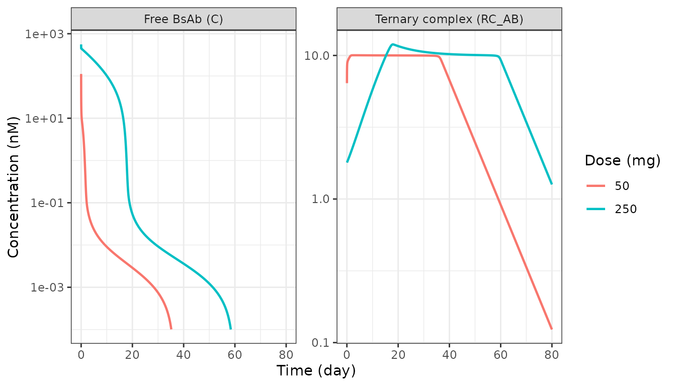
The paper’s three stated observations from this figure are checked numerically. The dose increases fivefold; the free-BsAb exposure increases by orders of magnitude while the trimer exposure barely moves, and the trimer peak is pushed far later.
auc_tr <- function(t, y) sum(diff(t) * (head(y, -1) + tail(y, -1)) / 2)

f3 <- fig3 |>
  group_by(dose_mg) |>
  summarise(
    auc_bsab = auc_tr(time, Cc),
    auc_trimer = auc_tr(time, trimer),
    tmax_trimer = time[which.max(trimer)],
    cmax_trimer = max(trimer),
    .groups = "drop"
  )

ratios <- tibble::tibble(
  Observation = c(
    "AUC ratio 250 mg / 50 mg, free BsAb",
    "AUC ratio 250 mg / 50 mg, trimer",
    "Trimer Tmax, 50 mg (day)",
    "Trimer Tmax, 250 mg (day)"
  ),
  `Paper (Results)` = c("~400x", "~1.5x", "immediate build-up", "delayed build-up"),
  Reproduced = c(
    sprintf("%.0fx", f3$auc_bsab[2] / f3$auc_bsab[1]),
    sprintf("%.2fx", f3$auc_trimer[2] / f3$auc_trimer[1]),
    sprintf("%.1f", f3$tmax_trimer[1]),
    sprintf("%.1f", f3$tmax_trimer[2])
  )
)
knitr::kable(ratios)| Observation | Paper (Results) | Reproduced |
|---|---|---|
| AUC ratio 250 mg / 50 mg, free BsAb | ~400x | 263x |
| AUC ratio 250 mg / 50 mg, trimer | ~1.5x | 1.36x |
| Trimer Tmax, 50 mg (day) | immediate build-up | 2.8 |
| Trimer Tmax, 250 mg (day) | delayed build-up | 18.0 |
stopifnot(
  # (i) free-BsAb exposure scales enormously more than trimer exposure.
  f3$auc_bsab[2] / f3$auc_bsab[1] > 100,
  f3$auc_trimer[2] / f3$auc_trimer[1] < 2,
  # (ii) the larger dose delays the trimer peak by at least fivefold.
  f3$tmax_trimer[2] > 5 * f3$tmax_trimer[1],
  # (iii) despite a 5x dose, peak trimer rises by well under twofold: the
  #       trimer is close to saturated already at 50 mg.
  f3$cmax_trimer[2] / f3$cmax_trimer[1] < 2
)
The trimer AUC ratio reproduces the paper’s “1.5 times” closely (1.36). The free-BsAb AUC ratio is of the paper’s stated order but not its exact figure; see Errata.
Figure 4: all six species
Replicates Figure 4 of Schropp 2019: a large (500 mg) i.v. bolus, showing the two linear-then-nonlinear elimination phases of the free BsAb and the two inflection points that mark recovery of each target.
fig4 <- solve_full(500, tmax = 120, by = 0.05)

fig4 |>
  transmute(time,
    `C (free BsAb)` = Cc, `R_A` = target_a, `R_B` = target_b,
    `RC_A` = complex_a, `RC_B` = complex_b, `RC_AB` = trimer
  ) |>
  pivot_longer(-time, names_to = "species", values_to = "conc") |>
  filter(conc > 1e-3) |>
  ggplot(aes(time, conc, colour = species)) +
  geom_line(linewidth = 0.8) +
  scale_y_log10() +
  labs(x = "Time (day)", y = "Concentration (nM)", colour = NULL) +
  theme_bw()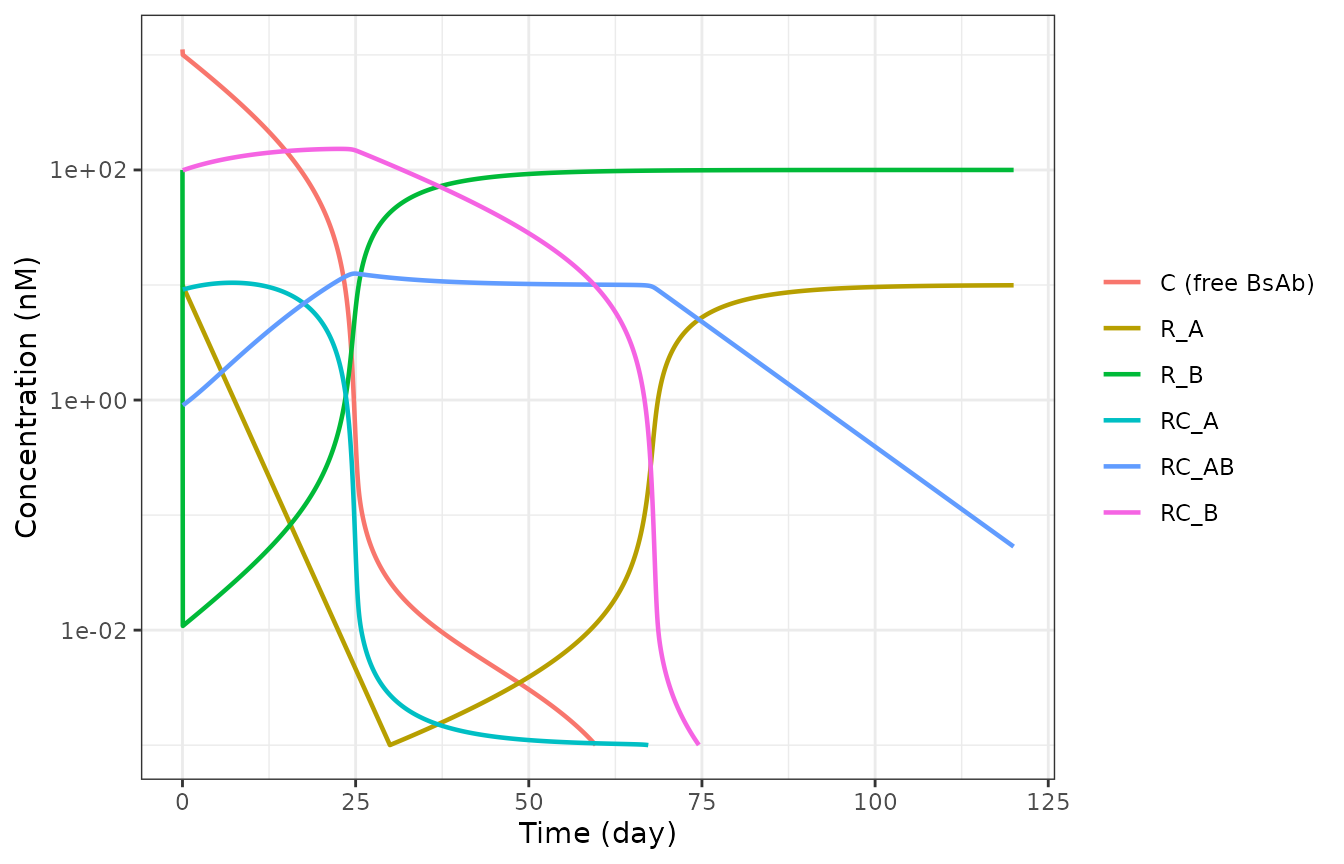
Both free receptors recover to their drug-free baselines, which the model file sets from the turnover steady state of Eq 9.
recovery <- tibble::tibble(
  Receptor = c("R_A", "R_B"),
  `Baseline from Eq 9 (nM)` = c(1 / 0.1, 10 / 0.1),
  `Value at t = 120 d (nM)` = c(tail(fig4$target_a, 1), tail(fig4$target_b, 1)),
  `Nadir (nM)` = c(min(fig4$target_a), min(fig4$target_b))
)
knitr::kable(recovery, digits = 3)| Receptor | Baseline from Eq 9 (nM) | Value at t = 120 d (nM) | Nadir (nM) |
|---|---|---|---|
| R_A | 10 | 9.947 | 0.000 |
| R_B | 100 | 99.993 | 0.011 |
Figure 2a: the bell-shaped total-drug / trimer relationship
The equilibrium-binding relationship of Eqs 20-22 and 26-30 is
exactly the algebra carried inside
Schropp_2019_bsab_tmdd_qeconst, so it can be evaluated
directly as a function of free BsAb concentration without solving an
ODE. Replicates Figure 2a of Schropp 2019, using that figure’s own
parameter settings: K_D1 = K_D2 = 0.01 nM,
RtotA = 10 nM, RtotB = 100 nM,
alpha = 1.
eb_curve <- function(C, kd1, kd2, alpha, rtota0, rtotb0) {
  qa <- (1 + C / kd2) * (C / (alpha * kd1 * kd2))
  qb <- (C * (rtota0 - rtotb0)) / (alpha * kd1 * kd2) + (1 + C / kd1) * (1 + C / kd2)
  qd <- -rtotb0 * (1 + C / kd1)
  rb <- ifelse(C > 0, (-qb + sqrt(qb^2 - 4 * qa * qd)) / (2 * qa), rtotb0)
  ra <- rtota0 / (1 + C / kd1 + rb * C / (alpha * kd1 * kd2))
  trimer <- C * ra * rb / (alpha * kd1 * kd2)
  tibble::tibble(
    C = C, RA = ra, RB = rb,
    complexA = C * ra / kd1, complexB = C * rb / kd2, trimer = trimer,
    Ctot = C + C * ra / kd1 + C * rb / kd2 + trimer
  )
}

eb <- eb_curve(10^seq(-6, 6, length.out = 2000),
  kd1 = 0.01, kd2 = 0.01, alpha = 1, rtota0 = 10, rtotb0 = 100
)

ggplot(eb, aes(Ctot, trimer)) +
  geom_line(linewidth = 0.8) +
  geom_vline(xintercept = c(10, 100), linetype = "dashed") +
  scale_x_log10() +
  labs(
    x = "Total BsAb concentration Ctot (nM)", y = "Ternary complex RC_AB (nM)",
    caption = "Dashed bars: the optimal working range of Eq 36"
  ) +
  theme_bw()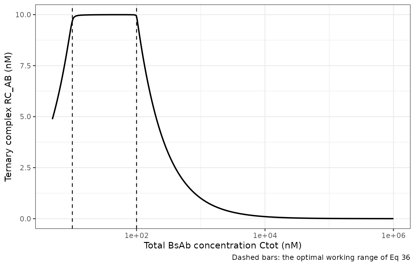
Three printed claims are checked. Eq 35 says the trimer vanishes as the BsAb concentration grows without bound; Eq 36 says the trimer is maximal while total drug lies between the two total receptor concentrations.
peak <- eb[which.max(eb$trimer), ]
claims <- tibble::tibble(
  Claim = c(
    "Eq 35: trimer -> 0 as C -> infinity",
    "Eq 36: Ctot at peak trimer lies in [min(RtotA,RtotB), max(RtotA,RtotB)] = [10, 100]",
    "Binary complexes saturate at RtotA and RtotB (text following Eq 35)"
  ),
  Reproduced = c(
    sprintf("trimer at C = 1e6 nM is %.3g nM (peak %.3g nM)", tail(eb$trimer, 1), peak$trimer),
    sprintf("Ctot at peak = %.1f nM", peak$Ctot),
    sprintf("max RC_A = %.3f (RtotA = 10), max RC_B = %.3f (RtotB = 100)", max(eb$complexA), max(eb$complexB))
  )
)
knitr::kable(claims)| Claim | Reproduced |
|---|---|
| Eq 35: trimer -> 0 as C -> infinity | trimer at C = 1e6 nM is 0.001 nM (peak 10 nM) |
| Eq 36: Ctot at peak trimer lies in [min(RtotA,RtotB), max(RtotA,RtotB)] = [10, 100] | Ctot at peak = 54.9 nM |
| Binary complexes saturate at RtotA and RtotB (text following Eq 35) | max RC_A = 9.999 (RtotA = 10), max RC_B = 99.999 (RtotB = 100) |
The QE approximation converges onto the full model
The paper states the defining property of the approximation: because
the QE model depends only on the ratios
K_DZ = k_offZ / k_onZ, scaling k_on and
k_off together (holding every K_D fixed)
drives the full model onto the QE approximation.
This is the strongest available check on both transcriptions at once. Two independently typed sets of equations – eight mass-action ODEs on one side, a 3x3 matrix of rational functions from Table 1 on the other – have no reason to agree unless both are right.
tob <- c(0.001, seq(0.05, 60, by = 0.05))
sq <- rxode2::rxSolve(
  qe,
  rxode2::et(amt = 50 * MG_TO_NMOL, cmt = "depot_iv", time = 0) |>
    rxode2::et(tob, cmt = "central"),
  params = NO_PERIPHERAL, omega = NA, sigma = NA,
  returnType = "data.frame", atol = 1e-14, rtol = 1e-12
)

conv <- lapply(c(1, 10, 100, 1000), function(s) {
  p <- c(NO_PERIPHERAL,
    lkon1 = log(10 * s), lkoff1 = log(0.01 * s),
    lkon2 = log(1 * s), lkoff2 = log(0.01 * s)
  )
  sf <- solve_full(50, tmax = 60, by = 0.05, params = p)
  d <- inner_join(
    select(sf, time, Cf = Cc, Tf = trimer),
    select(sq, time, Cq = Cc, Tq = trimerAB),
    by = "time"
  ) |>
    filter(time >= 0.5, Cf > LLOQ)
  tibble::tibble(
    `k_on, k_off scaling` = s,
    `Free BsAb max % difference` = max(abs(100 * (d$Cq - d$Cf) / d$Cf)),
    `Trimer max % difference` = max(abs(100 * (d$Tq - d$Tf) / d$Tf))
  )
}) |>
  bind_rows()

knitr::kable(conv, digits = 3)| k_on, k_off scaling | Free BsAb max % difference | Trimer max % difference |
|---|---|---|
| 1 | 72.652 | 1.768 |
| 10 | 20.020 | 0.318 |
| 100 | 2.271 | 0.044 |
| 1000 | 0.187 | 0.003 |
stopifnot(
  # Monotone convergence in both species.
  all(diff(conv$`Free BsAb max % difference`) < 0),
  all(diff(conv$`Trimer max % difference`) < 0),
  # At 1000x the two models agree to well under 1%.
  conv$`Free BsAb max % difference`[4] < 1,
  conv$`Trimer max % difference`[4] < 0.05,
  # At the paper's own (modest) binding rates the trimer already agrees closely,
  # which is why the approximation is useful even though free drug does not.
  conv$`Trimer max % difference`[1] < 5
)
At the paper’s own binding rates the two models disagree materially
in free BsAb while agreeing closely in the trimer,
which is the species that matters. This is consistent with the paper’s
remark that “depending on (i) inclusion of a peripheral compartment,
(ii) route of administration, and (iii) dose amount, large values of
k_onX, k_offX may be needed”.
The constant-total-receptor reduction holds its totals constant
Schropp_2019_bsab_tmdd_qeconst replaces two receptor
ODEs by the algebra of Eqs 26-30, under the assumption of Eq 23. If that
algebra is transcribed correctly the two total receptor pools
must stay pinned at their baselines for all time, for any dose. This is
a structural identity, so it is asserted tightly.
tobs <- c(0.001, seq(0.05, 120, by = 0.05))
qc <- rxode2::rxSolve(
  qeconst,
  rxode2::et(amt = 250 * MG_TO_NMOL, cmt = "depot_iv", time = 0) |>
    rxode2::et(tobs, cmt = "Cc"),
  omega = NA, sigma = NA, returnType = "data.frame", atol = 1e-14, rtol = 1e-12
) |>
  distinct(time, .keep_all = TRUE) |>
  mutate(RtotA = RA + complexA + trimerAB, RtotB = RB + complexB + trimerAB)

tibble::tibble(
  Pool = c("R_totA", "R_totB"),
  `Eq 23 value (nM)` = c(10, 100),
  `Simulated min` = c(min(qc$RtotA), min(qc$RtotB)),
  `Simulated max` = c(max(qc$RtotA), max(qc$RtotB))
) |>
knitr::kable(digits = 10)| Pool | Eq 23 value (nM) | Simulated min | Simulated max |
|---|---|---|---|
| R_totA | 10 | 10 | 10 |
| R_totB | 100 | 100 | 100 |
Figure 5a-c: the optimal dosing strategy
With constant total receptors and k_el = k_int, the
paper derives closed-form optimal doses and re-dosing times (Eqs 39-41).
Those formulas are evaluated here and then checked against the simulated
system.
R0A <- 10
R0B <- 100
kel <- 0.1

dose_init <- max(R0A, R0B) * VC / MG_TO_NMOL # Eq 39
dose_seq <- (max(R0A, R0B) - min(R0A, R0B)) * VC / MG_TO_NMOL # Eq 41
t_opt <- log(max(R0A, R0B) / min(R0A, R0B)) / kel # Eq 40

tibble::tibble(
  Quantity = c("Initial dose (Eq 39)", "Subsequent doses (Eq 41)", "Re-dosing interval (Eq 40)"),
  `Paper (Results)` = c("44.8 mg", "40.3 mg", "23 day"),
  Reproduced = c(
    sprintf("%.1f mg", dose_init), sprintf("%.1f mg", dose_seq), sprintf("%.1f day", t_opt)
  )
) |>
knitr::kable()| Quantity | Paper (Results) | Reproduced |
|---|---|---|
| Initial dose (Eq 39) | 44.8 mg | 44.8 mg |
| Subsequent doses (Eq 41) | 40.3 mg | 40.3 mg |
| Re-dosing interval (Eq 40) | 23 day | 23.0 day |
Now the regimen is simulated. The paper’s claim is that this schedule holds total drug inside the optimal working range, and therefore holds the trimer at its maximal achievable concentration, even though free BsAb falls below the LLOQ long before the next dose is due.
ev5 <- rxode2::et(amt = dose_init * MG_TO_NMOL, cmt = "depot_iv", time = 0)
for (k in 1:3) {
  ev5 <- rxode2::et(ev5, amt = dose_seq * MG_TO_NMOL, cmt = "depot_iv", time = k * t_opt)
}
# Sampling starts at 0.001 day, following the paper's own advice to shift a
# time-zero measurement slightly when an i.v. bolus is mimicked by a short
# infusion (Methods, "Implementation of the QE approximation with an i.v.
# administration").
ev5 <- rxode2::et(ev5, c(0.001, seq(0.02, 4 * t_opt, by = 0.02)), cmt = "Cc")

s5 <- rxode2::rxSolve(qeconst, ev5,
  omega = NA, sigma = NA,
  returnType = "data.frame", atol = 1e-14, rtol = 1e-12
) |>
  distinct(time, .keep_all = TRUE)

s5 |>
  transmute(time,
    `a: free BsAb C` = Cc, `b: total BsAb Ctot` = CcTotal,
    `c: ternary complex RC_AB` = trimerAB
  ) |>
  pivot_longer(-time, names_to = "panel", values_to = "conc") |>
  ggplot(aes(time, conc)) +
  geom_line(linewidth = 0.8) +
  geom_hline(
    data = tibble::tibble(panel = "b: total BsAb Ctot", y = c(10, 100)),
    aes(yintercept = y), linetype = "dashed"
  ) +
  geom_hline(
    data = tibble::tibble(panel = "a: free BsAb C", y = LLOQ),
    aes(yintercept = y), linetype = "dotted"
  ) +
  facet_wrap(~panel, ncol = 1, scales = "free_y") +
  scale_y_log10() +
  labs(x = "Time (day)", y = "Concentration (nM)") +
  theme_bw()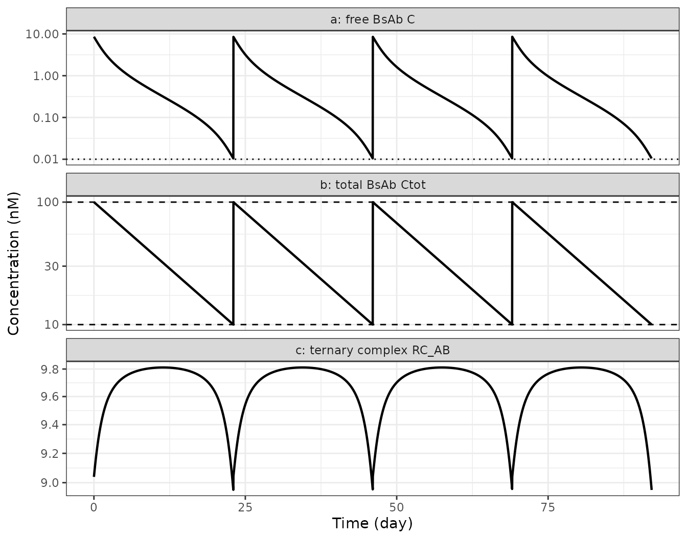
w <- filter(s5, time > 1e-3)
in_range <- mean(w$CcTotal >= R0A - 1e-6 & w$CcTotal <= R0B + 1e-6)
trimer_max_possible <- max(eb_curve(10^seq(-6, 6, length.out = 4000),
  kd1 = 0.1, kd2 = 1, alpha = 1, rtota0 = R0A, rtotb0 = R0B
)$trimer)

tibble::tibble(
  Claim = c(
    "C(0) is approximately 1 nM despite a 44.8 mg dose ('due to high affinity')",
    "Ctot stays within the optimal working range [10, 100] nM",
    "Ctot at t_opt returns to min(RtotA, RtotB) = 10 nM (Eq 40)",
    "Free BsAb is below the 0.01 nM LLOQ at the re-dosing time",
    "Trimer is held near its maximum achievable concentration"
  ),
  Reproduced = c(
    sprintf("C(0.001) = %.2f nM", s5$Cc[1]),
    sprintf("%.1f%% of the time; range %.2f-%.2f nM", 100 * in_range, min(w$CcTotal), max(w$CcTotal)),
    sprintf("%.2f nM", s5$CcTotal[which.min(abs(s5$time - t_opt))]),
    sprintf("C(t_opt) = %.4f nM", s5$Cc[which.min(abs(s5$time - t_opt))]),
    sprintf("min %.2f nM vs max achievable %.2f nM", min(w$trimerAB), trimer_max_possible)
  )
) |>
knitr::kable()| Claim | Reproduced |
|---|---|
| C(0) is approximately 1 nM despite a 44.8 mg dose (‘due to high affinity’) | C(0.001) = 8.56 nM |
| Ctot stays within the optimal working range [10, 100] nM | 100.0% of the time; range 10.00-99.98 nM |
| Ctot at t_opt returns to min(RtotA, RtotB) = 10 nM (Eq 40) | 10.01 nM |
| Free BsAb is below the 0.01 nM LLOQ at the re-dosing time | C(t_opt) = 0.0105 nM |
| Trimer is held near its maximum achievable concentration | min 8.95 nM vs max achievable 9.81 nM |
stopifnot(
  # Total drug never leaves the optimal working range.
  in_range > 0.999,
  min(w$CcTotal) >= R0A - 1e-3,
  max(w$CcTotal) <= R0B + 1e-3,
  # Eq 40 lands Ctot back on the lower edge of the window.
  abs(s5$CcTotal[which.min(abs(s5$time - t_opt))] - R0A) / R0A < 0.01,
  # The point of the paper: the trimer is held near its ceiling throughout.
  min(w$trimerAB) > 0.85 * trimer_max_possible
)
The free BsAb concentration spends most of the dosing interval below the assay LLOQ, yet the trimer is held within 9% of its ceiling. This is the paper’s practical conclusion: for a BsAb, an undetectable free-drug concentration does not imply an inactive system, so a re-dosing rule driven by free-drug PK would over-dose the patient.
PKNCA validation
Non-compartmental analysis of the free BsAb after the two Figure 3 doses. The paper reports no NCA table, so this section establishes the exposure metrics rather than comparing against published ones; the comparison that is available against published numbers is the AUC-ratio check above.
nca_conc <- fig3 |>
  filter(!is.na(Cc)) |>
  transmute(id = 1L, arm = factor(dose_mg), time, conc = Cc)

nca_dose <- fig3 |>
  distinct(dose_mg) |>
  transmute(id = 1L, arm = factor(dose_mg), time = 0, dose = dose_mg * MG_TO_NMOL)

o_conc <- PKNCA::PKNCAconc(nca_conc, conc ~ time | arm / id)
# PKNCAdose does not accept a nested (`/`) grouping formula; it takes the same
# grouping columns joined with `+`.
o_dose <- PKNCA::PKNCAdose(nca_dose, dose ~ time | arm + id)
res <- PKNCA::pk.nca(PKNCA::PKNCAdata(o_conc, o_dose))

nca_tab <- as.data.frame(res) |>
  filter(PPTESTCD %in% c("cmax", "tmax", "auclast", "half.life")) |>
  select(arm, PPTESTCD, PPORRES) |>
  pivot_wider(names_from = PPTESTCD, values_from = PPORRES)

nca_tab |>
  rename(
    "Dose (mg)" = arm, "Cmax (nM)" = cmax, "Tmax (day)" = tmax,
    "AUClast (nM*day)" = auclast, "t1/2 (day)" = half.life
  ) |>
knitr::kable(digits = 3)| Dose (mg) | AUClast (nM*day) | Cmax (nM) | Tmax (day) | t1/2 (day) |
|---|---|---|---|---|
| 50 | 10.453 | 111.667 | 0 | 6.669 |
| 250 | 2793.570 | 558.333 | 0 | 5.840 |
stopifnot(
  # An i.v. bolus peaks at the first sample in both arms.
  all(nca_tab$tmax <= 0.001),
  # Exposure is strongly MORE than dose-proportional: a 5x dose gives far more
  # than 5x AUC, the signature of saturable target-mediated elimination.
  nca_tab$auclast[nca_tab$arm == "250"] / nca_tab$auclast[nca_tab$arm == "50"] > 5 * 5
)
The grossly super-proportional AUC increase is the expected fingerprint of target-mediated elimination: at 50 mg most of the dose is bound and internalised through the receptors, while at 250 mg the receptors are saturated and the drug is left to clear linearly.
Simulation-estimation study (Table 2)
The paper’s identifiability study is reproduced as a table, not
re-run. Study 1 fitted free BsAb only and could not identify
K_D1 / K_D2; Study 2 added free receptor A and
B measurements and recovered them. alpha was fixed
throughout. The model file’s defaults are the true
values column.
tibble::tribble(
  ~Parameter, ~Units, ~`True value`, ~`MONOLIX study 1`, ~`NONMEM study 1`, ~`MONOLIX study 2`, ~`NONMEM study 2`,
  "k_el", "1/day", "0.1", "0.126", "0.118", "0.104", "0.104",
  "K_D1", "nM", "0.1", "0.1 (fixed)", "0.1 (fixed)", "0.114", "0.13",
  "K_D2", "nM", "1", "1 (fixed)", "1 (fixed)", "1.05", "1.04",
  "alpha", "-", "1 (fixed)", "1 (fixed)", "1 (fixed)", "1 (fixed)", "1 (fixed)",
  "R_A^0", "nM", "10", "7.05", "8.18", "9.78", "9.79",
  "R_B^0", "nM", "100", "78.3", "87.5", "100", "100",
  "k_int", "1/day", "0.1", "0.105", "0.103", "0.100", "0.100",
  "V", "L", "3", "2.73", "2.73", "2.84", "2.85",
  "omega_kel", "-", "0.05", "0.045", "0.049", "0.023", "0.010",
  "omega_V", "-", "0.05", "0.058", "0.056", "0.065", "0.066",
  "b1", "-", "0.2", "0.206", "0.205", "0.210", "0.211",
  "b2", "-", "0.2", "-", "-", "0.206", "0.206",
  "b3", "-", "0.2", "-", "-", "0.207", "0.207"
) |>
knitr::kable()| Parameter | Units | True value | MONOLIX study 1 | NONMEM study 1 | MONOLIX study 2 | NONMEM study 2 |
|---|---|---|---|---|---|---|
| k_el | 1/day | 0.1 | 0.126 | 0.118 | 0.104 | 0.104 |
| K_D1 | nM | 0.1 | 0.1 (fixed) | 0.1 (fixed) | 0.114 | 0.13 |
| K_D2 | nM | 1 | 1 (fixed) | 1 (fixed) | 1.05 | 1.04 |
| alpha | - | 1 (fixed) | 1 (fixed) | 1 (fixed) | 1 (fixed) | 1 (fixed) |
| R_A^0 | nM | 10 | 7.05 | 8.18 | 9.78 | 9.79 |
| R_B^0 | nM | 100 | 78.3 | 87.5 | 100 | 100 |
| k_int | 1/day | 0.1 | 0.105 | 0.103 | 0.100 | 0.100 |
| V | L | 3 | 2.73 | 2.73 | 2.84 | 2.85 |
| omega_kel | - | 0.05 | 0.045 | 0.049 | 0.023 | 0.010 |
| omega_V | - | 0.05 | 0.058 | 0.056 | 0.065 | 0.066 |
| b1 | - | 0.2 | 0.206 | 0.205 | 0.210 | 0.211 |
| b2 | - | 0.2 | - | - | 0.206 | 0.206 |
| b3 | - | 0.2 | - | - | 0.207 | 0.207 |
The inter-individual variability of the constant-total-receptor model
is exercised below with a cohort of 200 subjects, confirming that the
omega values encode as the paper’s standard
deviations (the model file stores
omega^2 = 0.05^2 = 0.0025).
set.seed(20260922)
rxode2::rxSetSeed(20260922)
N <- 200
ev_iiv <- rxode2::et(amt = 250 * MG_TO_NMOL, cmt = "depot_iv", time = 0) |>
  rxode2::et(c(0.001, seq(0.5, 40, by = 0.5)), cmt = "Cc")

s_iiv <- rxode2::rxSolve(qeconst, ev_iiv, nSub = N, returnType = "data.frame")

# The model applies each eta as exp(l<param> + eta<param>), so the realised
# between-subject SD of log(k_el) and log(V) IS the omega the paper reports.
# Checking the individual parameters rather than the eta draws also confirms the
# variability actually reaches the parameters.
subj <- distinct(s_iiv, sim.id, .keep_all = TRUE)

tibble::tibble(
  Quantity = c("Between-subject SD of log(k_el)", "Between-subject SD of log(V)"),
  `Paper true value (omega)` = c(0.05, 0.05),
  `Realised in a 200-subject cohort` = c(sd(log(subj$kel)), sd(log(subj$vc)))
) |>
knitr::kable(digits = 4)| Quantity | Paper true value (omega) | Realised in a 200-subject cohort |
|---|---|---|
| Between-subject SD of log(k_el) | 0.05 | 0.0541 |
| Between-subject SD of log(V) | 0.05 | 0.0520 |
stopifnot(
  # Medians sit on the typical values: the etas are mean-zero on the log scale.
  abs(median(subj$kel) - 0.1) / 0.1 < 0.05,
  abs(median(subj$vc) - 3) / 3 < 0.05,
  # The realised SD of a 200-draw sample is within sampling error of 0.05.
  # This is the check that the omegas are stored as VARIANCES (0.05^2) and not
  # as standard deviations -- the latter would give a realised SD near 0.22.
  abs(sd(log(subj$kel)) - 0.05) < 0.02,
  abs(sd(log(subj$vc)) - 0.05) < 0.02
)
Assumptions and deviations
-
No population, no drug, no covariates. This is a
theoretical paper. Every
ini()value isfixed(), matching the authors’ own all-FIXcontrol streams (S4-S6, S8-S10). - Three model files, one per structural variant. The paper presents the full model, the QE approximation with non-constant total receptors, and the QE approximation with constant total receptors as three distinct models, and gives each its own MONOLIX and NONMEM control stream. They are therefore extracted as three files rather than one parameterised file.
-
The equilibrium-binding (EB) model is not a fourth
file. It is the QE model with turnover, elimination and
internalisation switched off, i.e. pure algebra with no differential
equation. It is reproduced in this vignette as the function
eb_curve(), which is the same algebraqeconstcarries internally. -
i.v. dosing through a dummy compartment. Under
rapid binding the i.v. input function is multiplied into the right-hand
side (Eqs 16-19, 25), so an i.v. dose cannot be added to the central
state. The paper devotes a Methods subsection to this and offers two
workarounds; the model files implement the dummy-compartment form of its
Eq 42, with the drain rate
kdum = 1/TDURset from the authors’ ownTDUR = 0.0001day. An i.v. dose must be given intodepot_iv, not intocentral, for both QE models. The full model is unaffected and takes an ordinary bolus intocentral. -
Mixed concentration and amount states.
centralholds a concentration whileperipheral1,depot_scanddepot_ivhold amounts. This reproduces the published equations and the authors’ NONMEM code exactly rather than renormalising them. -
alpha = 1throughout. The paper fixesalphain every fit and states that its Table 2 simplification (k_on3 = k_on2etc.) is equivalent toalpha = 1. No non-unity value is reported anywhere, so none is encoded. -
QE model defaults are converted, not transcribed.
K_D1 = 0.001nM andK_D2 = 0.01nM are computed from the Table 2k_off/k_onpairs. The conversion is confirmed by the authors’ own S5 stream, which hard-codes those two numbers. -
qeconstcarries no peripheral compartment. This matches the authors’ S10 (NCOMP=1) and the paper’s statement that “for simplicity, the peripheral compartment was neglected” in the Figure 5a-c example. The paper’s peripheral-plus-s.c. example (Figure 5d-f) uses the full model, which is available. -
qeconstdefaults are the true, not the fitted, values. The four fitted columns disagree with one another in the third significant figure and two of them carry fixedK_Ds; the data-generating values are the authoritative set. All four columns are tabulated above.
Errata and unresolved points
- Free-BsAb AUC ratio. The Results section states that between the 50 mg and 250 mg doses of Figure 3 the free-BsAb AUC differs by “400 times” while the trimer AUC differs by “1.5 times”. The trimer figure reproduces closely (1.36), but the free-BsAb ratio reproduces as 263 rather than 400. The paper does not state the integration window, and the free-BsAb AUC at 50 mg is small and dominated by the first hours after the bolus, so this ratio is very sensitive to where integration starts and stops (the paper also imposes a 0.01 nM LLOQ). The qualitative claim – that free-drug exposure scales with dose by orders of magnitude while trimer exposure barely moves – reproduces robustly and is what the assertion above tests.
-
Residual error and IIV for the full model are not
reported. The full model is used only for simulation; its
NONMEM stream S6 has
$ESTIMATIONcommented out and carries a placeholder proportional error fixed at 1 with all$OMEGAat0 FIX.propSdis therefore encoded asfixed(0)rather than inventing a value. The only residual errors and IIV the paper estimates belong to the simulation-estimation study and are carried byqeconst. -
Figure 2 panels b-e are not reproduced. They are
parameter sweeps whose swept ranges are shown graphically but not
tabulated.
eb_curve()is exposed above so a reader can reproduce any of them directly. - Equation images. The published PDF’s display equations do not survive text extraction. Every structural equation used here was read from the PDF text layer and then cross-checked line by line against the authors’ NONMEM source in Supplementary Material S5, S6, S9 and S10, which is the same mathematics written in FORTRAN and is unambiguous.