Whole-body aging physiology, 30 to 100 years (Schlender 2016)
Source:vignettes/articles/Schlender_2016_aging_physiology.Rmd
Schlender_2016_aging_physiology.RmdModel and source
- Citation: Schlender JF, Meyer M, Thelen K, Krauss M, Willmann S, Eissing T, Jaehde U. Development of a Whole-Body Physiologically Based Pharmacokinetic Approach to Assess the Pharmacokinetics of Drugs in Elderly Individuals. Clin Pharmacokinet. 2016;55(12):1573-1589. doi:10.1007/s40262-016-0422-3.
- Article: https://doi.org/10.1007/s40262-016-0422-3
- Supplement (Springer ESM, open access): https://doi.org/10.1007/s40262-016-0422-3
Schlender 2016 is not a drug model. It is the system layer that a whole-body physiologically based pharmacokinetic (PBPK) model sits on, extended for the first time across the full course of healthy aging to 100 years of age. The paper’s deliverable is an age- and sex-resolved description of human physiology: body weight and height, thirteen organ and tissue masses, the cardiac index, ten organ blood flow rates, and a new aging function for the glomerular filtration rate (GFR).
That system layer is what this package extracts. Everything in it is published as numbers – Tables 2 and 3 and Equation 1 – and is reproduced here exactly.
What is deliberately not extracted, and why
Schlender 2016 verifies its physiology by building PBPK models of two intravenously dosed probe drugs, morphine (high hepatic extraction) and furosemide (mainly renal), in PK-Sim v5.5. Those two drug models are not part of this extraction, because they are not reproducible from the paper:
- Table 1 is a compound card (molecular weight, log P, pKa, fraction unbound, specific clearances) – the inputs to the platform, not the model.
- The tissue:plasma partition coefficients and the cellular permeabilities, which are the drug-specific parameters a whole-body PBPK actually runs on, are given only as a named method (“Willmann et al., defined as the PK-Sim standard”). A named method is an algorithm, not a set of values.
- No PK-Sim project file was deposited, and the supplement contains only the aging-physiology literature review and Supplement Table 1 (the list of studies) – it holds no partition coefficients, no permeabilities and no ODEs.
Counting what would be needed against what is printed, the drug layer scores roughly 5 published parameters out of 35+ required per compound. The physiology layer, by contrast, is complete and is verified below.
Users who want a morphine or furosemide PK model to pair with this
physiology can chain an independent compartmental model already in the
registry, for example Elkomy_2015_morphine,
Knibbe_2009_morphine or
Hornik_2025_furosemide, or the PK-Sim-independent
Gu_2025_furosemide_pbpk.
Population
- Species: human
- Age range: 30 to 100 years (the aging model; the underlying PK-Sim adult model extends below 30 y, and Fig. 2 shows organ weights from newborns, but the trajectories extracted here are defined on the 30-100 y decade knots of Tables 2 and 3)
- Race / ethnicity: Healthy European Caucasians. Where European data were too sparse to describe an organ across the full age range, North American and Australian data were added (Methods, Workflow for Elderly PBPK Model Development; Discussion)
- Regions: Europe, with North American and Australian data added for sparsely reported organs and for blood flow / cardiac output
The physiology is assembled from a literature analysis, not from a single cohort: 19 studies carried over from the Thompson et al. database plus 97 studies added by this paper’s own two PubMed / Google Scholar / MedPilot searches (Methods). Inclusion required clear assignment of sex and race, a comprehensible statement of the method of analysis, and exclusion of medication or disease effects on physiology; longitudinal surveillance was preferred. Organ volumes came mostly from autopsy series, with in vivo measurements used only for muscle, fat and blood flow.
The GFR aging function of Equation 1 was fitted to body-surface-area-adjusted data from 1,213 females and 1,081 males, mostly prospective renal transplant donors assessed with exogenous markers (Results, Glomerular Filtration Rate).
For the physiological-consistency checks the paper created a virtual 30-year-old in PK-Sim v5.5 and generated a virtual population of N = 5,000 for each sex over 30 to 100 years.
The same information is available programmatically via
readModelDb("Schlender_2016_aging_physiology")()$population.
Source trace
The per-parameter origin is recorded as an in-file comment next to
each ini() entry in
inst/modeldb/endogenous/Schlender_2016_aging_physiology.R.
The table below collects the whole model in one place.
| Model component | Source location |
|---|---|
bw, ht
|
Table 2, rows “Body weight, kg” and “Height, cm” (female + male) |
mass_blood, mass_bone,
mass_brain, mass_fat,
mass_gonads, mass_heart,
mass_kidney, mass_liver,
mass_lung, mass_muscle,
mass_pancreas, mass_skin,
mass_spleen
|
Table 2, “Organ masses, g” (female + male) |
mass_gi |
Table 2 footnote a: held constant at 1274.5 g (female) / 1304.8 g (male) |
cardiac_index |
Table 3, row “Cardiac index, L/m2” (female + male) |
flow_adipose, flow_cerebral,
flow_gonads, flow_myocardial,
flow_renal, flow_splanchnic,
flow_hepatic, flow_muscle,
flow_skeleton, flow_skin
|
Table 3, “Organ blood flow, mL/min” (female + male) |
| Linear interpolation between decade knots | Methods, “Workflow for Elderly PBPK Model Development”: data pooled into 10-year age bins “and interpolated linearly” |
gfr_fpma = 26.6 mL/min/100 g |
Text below Equation 1 (Rhodin maturation function at full maturation, 40th gestational week) |
gfr_vmax = 0.9 |
Text below Equation 1, “maximal decreasing rate factor” |
gfr_ta50_female = 59 y, gfr_ta50_male = 54
y |
Text below Equation 1, “aging half-time” |
gfr_hill = 1.5 |
Text below Equation 1, “The Hill coefficient was parameterized at 1.5” |
gfr_specific, gfr
|
Equation 1, page 1581 |
Equation 1 is an embedded image in the published PDF
and is dropped by every text converter (it does not survive plain-text
extraction of the PDF and is absent from pdftotext output).
It was recovered from the publisher’s equation graphic
(40262_2016_422_Article_Equ1.gif, deposited with the
article, PMC5107207) and confirmed by rendering page 8 of the PDF at 400
dpi. As printed:
Units
The model has no ODEs, so the dimensional check is on the algebraic outputs.
| Symbol | Units | Note |
|---|---|---|
time / age
|
year | the rxode2 time variable is chronological age |
bw |
kg | |
ht |
cm | |
mass_* |
g | including mass_gi, which is age-invariant |
cardiac_index |
L/min/m^2 | Table 3 prints the header as “L/m2”; the cardiac index is a flow per unit BSA, so the per-minute is implicit |
bsa |
m^2 | Du Bois, from ht (cm) and bw (kg) |
cardiac_output |
mL/min |
cardiac_index (L/min/m^2) x bsa (m^2) x
1000 (mL/L) |
flow_* |
mL/min | |
gfr_fpma, gfr_specific
|
mL/min per 100 g kidney | |
gfr_ta50_*, gfr_age
|
year | |
gfr_vmax, gfr_hill
|
unitless | see Errata on the gfr_vmax unit tag |
gfr |
mL/min |
gfr_specific (mL/min/100 g) x mass_kidney
(g) / 100 |
Parameter table
| Parameter | Value | Fixed in source | Label |
|---|---|---|---|
| gfr_fpma | 26.6 | TRUE | Specific GFR after full maturation F_PMA (mL/min per 100 g kidney weight) |
| gfr_vmax | 0.9 | TRUE | Maximal fractional decrease in specific GFR with aging Vmax (fraction of F_PMA) |
| gfr_ta50_female | 59.0 | TRUE | Aging half-time TA50 for females (years after the age of 30) |
| gfr_ta50_male | 54.0 | TRUE | Aging half-time TA50 for males (years after the age of 30) |
| gfr_hill | 1.5 | TRUE | Hill coefficient of the GFR aging function (unitless) |
All five are published point estimates of a fitted function with no
reported standard error, so all are fixed().
Simulation
The model is deterministic: no between-subject variability and no residual error are encoded (see Errata). One “subject” per sex is solved across the full published age range.
mod <- readModelDb("Schlender_2016_aging_physiology")

solve_sex <- function(sexf, ages) {
  ev <- as.data.frame(rxode2::et(ages))
  ev$SEXF <- sexf
  out <- rxode2::rxSolve(mod, ev, returnType = "data.frame")
  out$SEXF <- sexf
  out$sex <- ifelse(sexf == 1, "Female", "Male")
  out
}

knots <- seq(30, 100, by = 10)
fine <- seq(30, 100, by = 0.5)

sim_knot <- dplyr::bind_rows(solve_sex(1, knots), solve_sex(0, knots))
sim_fine <- dplyr::bind_rows(solve_sex(1, fine), solve_sex(0, fine))

nrow(sim_knot)
#> [1] 16
nrow(sim_fine)
#> [1] 282
Validation
1. Exact reproduction of Tables 2 and 3
The strongest available gate: the model must return every one of the 416 published cells of Tables 2 and 3 at the decade knots. The reference values below are transcribed independently from the article PDF.
# Schlender 2016 Table 2 (anthropometry + organ masses) and Table 3
# (cardiac index + organ blood flows). Order is age 30, 40, ..., 100.
ref <- tibble::tribble(
  ~var, ~sex, ~v30, ~v40, ~v50, ~v60, ~v70, ~v80, ~v90, ~v100,
  # ---- Table 2 ----
  "bw", "Female", 60.0, 63.3, 65.2, 65.5, 62.2, 56.1, 53.7, 45.2,
  "bw", "Male", 73.0, 74.4, 73.0, 72.0, 71.1, 68.1, 64.9, 55.6,
  "ht", "Female", 163.0, 160.9, 160.0, 158.3, 155.4, 151.7, 150.0, 147.9,
  "ht", "Male", 176.0, 175.1, 173.9, 171.2, 167.4, 165.5, 163.8, 157.6,
  "mass_blood", "Female", 1899.4, 1921.1, 1961.2, 1946.9, 1847.7, 1692.6, 1634.5, 1357.0,
  "mass_blood", "Male", 2264.6, 2269.5, 2234.9, 2180.2, 2111.3, 2042.5, 1976.5, 1739.5,
  "mass_bone", "Female", 9121.5, 8886.3, 8676.1, 8401.8, 7811.6, 6981.4, 6619.0, 6263.5,
  "mass_bone", "Male", 11817.8, 11848.0, 11481.6, 11091.6, 10355.0, 9637.1, 8969.0, 8300.9,
  "mass_brain", "Female", 1357.0, 1352.3, 1347.6, 1315.1, 1287.3, 1241.4, 1169.4, 1097.4,
  "mass_brain", "Male", 1508.8, 1506.9, 1502.9, 1463.3, 1434.3, 1400.1, 1372.1, 1344.2,
  "mass_fat", "Female", 19348.0, 20002.5, 23815.4, 26993.0, 27884.7, 25694.5, 25020.6, 20171.4,
  "mass_fat", "Male", 14868.0, 16309.7, 16676.5, 17920.7, 19447.4, 19947.7, 20691.0, 17082.3,
  "mass_gonads", "Female", 13.1, 13.0, 6.6, 5.3, 5.2, 5.1, 5.1, 4.9,
  "mass_gonads", "Male", 40.3, 40.8, 35.0, 33.5, 31.9, 30.6, 30.3, 29.5,
  "mass_heart", "Female", 328.4, 340.0, 355.6, 377.1, 399.1, 413.5, 431.2, 412.9,
  "mass_heart", "Male", 417.2, 434.3, 439.1, 454.6, 464.8, 441.4, 437.9, 425.1,
  "mass_kidney", "Female", 403.4, 401.7, 400.5, 383.4, 364.2, 325.2, 308.8, 295.8,
  "mass_kidney", "Male", 437.7, 475.9, 468.1, 455.6, 441.7, 395.7, 366.7, 355.9,
  "mass_liver", "Female", 1905.5, 1881.0, 1867.7, 1679.8, 1504.9, 1423.4, 1329.5, 1189.4,
  "mass_liver", "Male", 2357.8, 2324.5, 2206.0, 2041.3, 1714.6, 1417.3, 1324.0, 1202.0,
  "mass_lung", "Female", 1009.5, 1021.4, 1038.8, 1023.8, 1005.4, 849.1, 804.5, 637.3,
  "mass_lung", "Male", 1294.3, 1334.7, 1337.4, 1349.0, 1271.8, 1138.0, 1007.4, 978.0,
  "mass_muscle", "Female", 20276.2, 23058.3, 21300.1, 18971.2, 15746.4, 13367.8, 12394.3, 10060.6,
  "mass_muscle", "Male", 32338.6, 32318.2, 31180.6, 29600.0, 28562.1, 26524.8, 23657.0, 19534.0,
  "mass_pancreas", "Female", 169.5, 170.3, 163.8, 158.7, 148.5, 131.9, 128.0, 122.6,
  "mass_pancreas", "Male", 190.3, 190.8, 183.6, 178.2, 165.4, 149.9, 143.7, 139.5,
  "mass_skin", "Female", 2723.5, 2773.2, 2836.2, 2829.5, 2725.8, 2559.1, 2493.8, 2223.5,
  "mass_skin", "Male", 3760.9, 3790.2, 3745.1, 3692.0, 3635.2, 3537.0, 3439.7, 3122.6,
  "mass_spleen", "Female", 219.2, 197.7, 190.7, 182.4, 164.5, 149.7, 99.4, 78.7,
  "mass_spleen", "Male", 243.4, 221.9, 208.2, 197.0, 186.6, 160.4, 133.4, 108.4,
  # ---- Table 3 ----
  "cardiac_index", "Female", 3.34, 3.33, 3.08, 2.89, 2.75, 2.68, 2.52, 2.41,
  "cardiac_index", "Male", 3.23, 3.22, 3.09, 2.86, 2.58, 2.36, 2.18, 2.04,
  "flow_adipose", "Female", 501.1, 528.2, 578.0, 655.3, 684.7, 630.2, 607.0, 491.5,
  "flow_adipose", "Male", 324.7, 352.1, 357.3, 381.4, 408.0, 419.8, 429.2, 357.3,
  "flow_cerebral", "Female", 707.8, 686.9, 666.1, 632.1, 601.2, 562.8, 514.2, 467.6,
  "flow_cerebral", "Male", 779.7, 747.6, 727.9, 692.9, 650.6, 623.8, 594.4, 536.1,
  "flow_gonads", "Female", 1.2, 1.2, 0.6, 0.5, 0.5, 0.5, 0.5, 0.4,
  "flow_gonads", "Male", 3.2, 3.3, 2.8, 2.7, 2.6, 2.5, 2.4, 2.4,
  "flow_myocardial", "Female", 295.0, 311.2, 313.2, 363.1, 376.3, 445.8, 464.8, 445.2,
  "flow_myocardial", "Male", 260.1, 271.1, 278.0, 299.1, 308.7, 334.7, 332.1, 322.3,
  "flow_renal", "Female", 1121.0, 1061.8, 943.8, 825.8, 707.8, 589.8, 471.8, 353.8,
  "flow_renal", "Male", 1325.0, 1339.3, 1116.3, 913.3, 730.3, 567.3, 424.3, 301.3,
  "flow_splanchnic", "Female", 1239.0, 1254.3, 1187.2, 1015.3, 862.6, 771.5, 679.1, 570.5,
  "flow_splanchnic", "Male", 1235.0, 1241.9, 1237.7, 1056.7, 813.1, 610.6, 512.9, 413.5,
  "flow_hepatic", "Female", 383.4, 388.1, 367.3, 314.2, 266.9, 238.7, 210.1, 176.5,
  "flow_hepatic", "Male", 423.0, 425.4, 423.9, 361.9, 278.5, 209.1, 175.7, 141.6,
  "flow_muscle", "Female", 665.1, 774.8, 636.6, 568.4, 479.8, 405.6, 369.0, 298.8,
  "flow_muscle", "Male", 1105.7, 1086.8, 1036.8, 975.0, 922.3, 861.7, 751.9, 625.9,
  "flow_skeleton", "Female", 294.9, 287.3, 280.5, 271.6, 252.6, 225.7, 214.0, 202.5,
  "flow_skeleton", "Male", 324.9, 325.8, 315.7, 305.0, 284.7, 265.0, 246.6, 228.2,
  "flow_skin", "Female", 295.7, 301.1, 307.9, 307.2, 295.9, 277.8, 270.7, 241.4,
  "flow_skin", "Male", 325.1, 327.7, 323.8, 319.2, 314.3, 305.8, 297.4, 270.0
) |>
  tidyr::pivot_longer(
    # Name the age columns explicitly: starts_with("v") would also match
    # the `var` column and silently poison the pivot.
    cols = dplyr::all_of(paste0("v", seq(30, 100, by = 10))),
    names_to = "age", values_to = "published"
  ) |>
  dplyr::mutate(age = as.numeric(sub("^v", "", .data$age)))

nrow(ref)
#> [1] 416
got <- sim_knot |>
  dplyr::select(age = "time", "sex", dplyr::all_of(unique(ref$var))) |>
  tidyr::pivot_longer(
    cols = dplyr::all_of(unique(ref$var)),
    names_to = "var", values_to = "simulated"
  )

cmp <- ref |>
  dplyr::inner_join(got, by = c("var", "sex", "age")) |>
  dplyr::mutate(abs_diff = abs(.data$simulated - .data$published))

# The join must not silently drop rows -- a lost row would make the
# gate below pass vacuously.
stopifnot(
  nrow(cmp) == nrow(ref),
  nrow(cmp) == 416L,
  !anyNA(cmp$simulated)
)

# Deterministic algebra: the model must return the published cells to
# machine precision, not "close to" them.
stopifnot(max(cmp$abs_diff) < 1e-8)

c(cells = nrow(cmp), max_abs_diff = max(cmp$abs_diff))
#>        cells max_abs_diff
#> 4.160000e+02 3.637979e-12
All 416 published cells are returned exactly.
The constant gastrointestinal mass of Table 2 footnote a is checked separately because it has no age dimension:
gi <- sim_fine |>
  dplyr::group_by(.data$sex) |>
  dplyr::summarise(lo = min(.data$mass_gi), hi = max(.data$mass_gi), .groups = "drop")

stopifnot(
  # Age-invariant within each sex.
  all(abs(gi$hi - gi$lo) < 1e-8),
  abs(gi$lo[gi$sex == "Female"] - 1274.5) < 1e-8,
  abs(gi$lo[gi$sex == "Male"] - 1304.8) < 1e-8
)
gi
#> # A tibble: 2 × 3
#>   sex       lo    hi
#>   <chr>  <dbl> <dbl>
#> 1 Female 1274. 1274.
#> 2 Male   1305. 1305.
2. Interpolation behaviour between and beyond the knots
The paper interpolates linearly between the ten-year bins. Between knots the model must therefore sit exactly on the chord, and outside 30 to 100 years the trajectory is held flat rather than extrapolating the last decade’s slope.
mid <- dplyr::bind_rows(solve_sex(1, c(35, 45, 95)), solve_sex(0, c(35, 45, 95)))
kn <- sim_knot

chord <- function(v, sex, a) {
  lo <- kn[[v]][kn$sex == sex & kn$time == a - 5]
  hi <- kn[[v]][kn$sex == sex & kn$time == a + 5]
  (lo + hi) / 2
}

midpoint_err <- vapply(
  c("mass_liver", "mass_kidney", "flow_renal", "bw"),
  function(v) {
    max(abs(vapply(
      c(35, 45, 95),
      function(a) {
        max(abs(c(
          mid[[v]][mid$sex == "Female" & mid$time == a] - chord(v, "Female", a),
          mid[[v]][mid$sex == "Male" & mid$time == a] - chord(v, "Male", a)
        )))
      },
      numeric(1)
    )))
  },
  numeric(1)
)

stopifnot(max(midpoint_err) < 1e-8)

# Flat outside the published 30-100 y range.
outside <- dplyr::bind_rows(solve_sex(1, c(10, 25, 30, 100, 110)), solve_sex(0, c(10, 25, 30, 100, 110)))
flat_lo <- outside |> dplyr::filter(.data$time %in% c(10, 25, 30))
flat_hi <- outside |> dplyr::filter(.data$time %in% c(100, 110))
stopifnot(
  dplyr::n_distinct(round(flat_lo$mass_liver[flat_lo$sex == "Male"], 8)) == 1L,
  dplyr::n_distinct(round(flat_hi$mass_liver[flat_hi$sex == "Male"], 8)) == 1L
)

midpoint_err
#>   mass_liver  mass_kidney   flow_renal           bw
#> 0.000000e+00 5.684342e-14 0.000000e+00 0.000000e+00
3. Cardiac-output mass balance
The paper states plainly that “the sum of all blood flows should be equal to CO” (Methods), and that age-related changes in blood flow distribution were accounted for as changes in cardiac output. This is an internal-consistency gate on Table 3 that the paper never reports numerically.
flow_cols <- c(
  "flow_adipose", "flow_cerebral", "flow_gonads", "flow_myocardial",
  "flow_renal", "flow_splanchnic", "flow_hepatic", "flow_muscle",
  "flow_skeleton", "flow_skin"
)

balance <- sim_knot |>
  dplyr::mutate(
    sum_flows = rowSums(dplyr::across(dplyr::all_of(flow_cols))),
    ratio = .data$sum_flows / .data$cardiac_output
  ) |>
  dplyr::select(age = "time", "sex", "sum_flows", "cardiac_output", "ratio")

stopifnot(nrow(balance) == 16L)

# The residual absorbs the organs Schlender 2016 excludes from Table 3
# (the paper notes the modelled organ masses reach only 91-95 % of body
# weight), the 3-significant-figure rounding of the published cells, and
# the unstated choice of BSA formula. 5 % leaves room for all three and
# still goes red on a mis-transcribed flow, which would move a single
# organ's contribution by tens of percent.
stopifnot(max(abs(balance$ratio - 1)) < 0.05)

balance |>
  dplyr::mutate(dplyr::across(c("sum_flows", "cardiac_output"), ~ round(.x, 0)), ratio = round(.data$ratio, 4)) |>
  dplyr::rename(
    "Age (y)" = "age", "Sex" = "sex",
    "Sum of Table 3 flows (mL/min)" = "sum_flows",
    "Cardiac output (mL/min)" = "cardiac_output",
    "Ratio" = "ratio"
  ) |>
knitr::kable()| Age (y) | Sex | Sum of Table 3 flows (mL/min) | Cardiac output (mL/min) | Ratio |
|---|---|---|---|---|
| 30 | Female | 5504 | 5491 | 1.0024 |
| 40 | Female | 5595 | 5548 | 1.0084 |
| 50 | Female | 5281 | 5176 | 1.0204 |
| 60 | Female | 4954 | 4828 | 1.0259 |
| 70 | Female | 4528 | 4435 | 1.0211 |
| 80 | Female | 4148 | 4065 | 1.0206 |
| 90 | Female | 3801 | 3721 | 1.0215 |
| 100 | Female | 3248 | 3274 | 0.9922 |
| 30 | Male | 6106 | 6102 | 1.0007 |
| 40 | Male | 6121 | 6110 | 1.0018 |
| 50 | Male | 5820 | 5787 | 1.0057 |
| 60 | Male | 5307 | 5265 | 1.0080 |
| 70 | Male | 4713 | 4648 | 1.0140 |
| 80 | Male | 4200 | 4140 | 1.0146 |
| 90 | Male | 3767 | 3719 | 1.0129 |
| 100 | Male | 3199 | 3169 | 1.0094 |
The flows sum to cardiac output within 2.6 % at every one of the 16 age-by-sex cells, and within 0.2 % at the ICRP-derived 30-year reference. Table 3 is internally consistent.
4. The GFR aging function (Equation 1), replicating Figure 5
# At age 30 the aging term is exactly zero, so specific GFR must equal
# F_PMA and absolute GFR must equal F_PMA * kidney mass / 100.
at30 <- sim_knot |> dplyr::filter(.data$time == 30)
stopifnot(
  all(abs(at30$gfr_specific - 26.6) < 1e-10),
  all(abs(at30$gfr - 26.6 * at30$mass_kidney / 100) < 1e-10)
)

# Specific GFR is strictly decreasing across the published range, and the
# female half-time (59 y) is longer than the male (54 y), so at any age
# above 30 the female retains a larger FRACTION of F_PMA.
sf <- sim_fine |> dplyr::filter(.data$sex == "Female") |> dplyr::arrange(.data$time)
sm <- sim_fine |> dplyr::filter(.data$sex == "Male") |> dplyr::arrange(.data$time)
stopifnot(
  all(diff(sf$gfr_specific) < 0),
  all(diff(sm$gfr_specific) < 0),
  all(sf$gfr_specific[sf$time > 30] > sm$gfr_specific[sm$time > 30])
)

round(at30$gfr, 1)
#> [1] 107.3 116.4
ggplot2::ggplot(sim_fine, ggplot2::aes(.data$time, .data$gfr)) +
  ggplot2::geom_line(linewidth = 0.8) +
  ggplot2::facet_wrap(~sex) +
  ggplot2::scale_y_continuous(limits = c(0, NA)) +
  ggplot2::labs(
    x = "Age (years)",
    y = "Glomerular filtration rate (mL/min)"
  ) +
  ggplot2::theme_bw()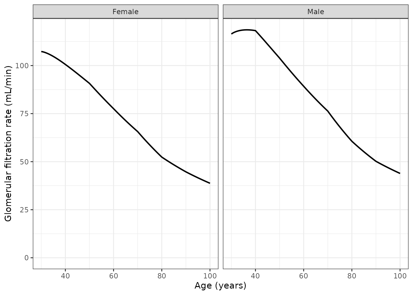
Replicates Figure 5 of Schlender 2016: absolute glomerular filtration rate over the course of aging, female (left) and male (right). The published panels show the fitted line falling from roughly 105 to 35 mL/min in females and from roughly 118 to 40 mL/min in males between 30 and 100 years.
gfr_ends <- sim_knot |>
  dplyr::filter(.data$time %in% c(30, 100)) |>
  dplyr::select(age = "time", "sex", "gfr_specific", "gfr")

# Read off the published Fig. 5 panels: the fitted GFR line starts near
# 105 (female) / 118 (male) mL/min at age 30 and ends near 35 / 40 at age
# 100. The model is the paper's own equation applied to the paper's own
# kidney masses, so agreement should be within the precision of reading a
# published axis -- 8 mL/min is about one third of a minor gridline.
fig5 <- c("Female_30" = 105, "Male_30" = 118, "Female_100" = 35, "Male_100" = 40)
key <- paste(gfr_ends$sex, gfr_ends$age, sep = "_")
stopifnot(all(key %in% names(fig5)))
stopifnot(max(abs(gfr_ends$gfr - fig5[key])) < 8)

gfr_ends |>
  dplyr::mutate(
    read_from_fig5 = fig5[paste(.data$sex, .data$age, sep = "_")],
    dplyr::across(c("gfr_specific", "gfr"), ~ round(.x, 1))
  ) |>
  dplyr::rename(
    "Age (y)" = "age", "Sex" = "sex",
    "Specific GFR (mL/min/100 g)" = "gfr_specific",
    "GFR (mL/min)" = "gfr",
    "Read from published Fig. 5" = "read_from_fig5"
  ) |>
knitr::kable()| Age (y) | Sex | Specific GFR (mL/min/100 g) | GFR (mL/min) | Read from published Fig. 5 |
|---|---|---|---|---|
| 30 | Female | 26.6 | 107.3 | 105 |
| 100 | Female | 13.1 | 38.8 | 35 |
| 30 | Male | 26.6 | 116.4 | 118 |
| 100 | Male | 12.3 | 43.9 | 40 |
5. Replicating Figure 3 (body height) and Figure 2 (organ masses)
ggplot2::ggplot(sim_fine, ggplot2::aes(.data$time, .data$ht, colour = .data$sex)) +
  ggplot2::geom_line(linewidth = 0.8) +
  ggplot2::labs(x = "Age (years)", y = "Body height (cm)", colour = "Sex") +
  ggplot2::theme_bw()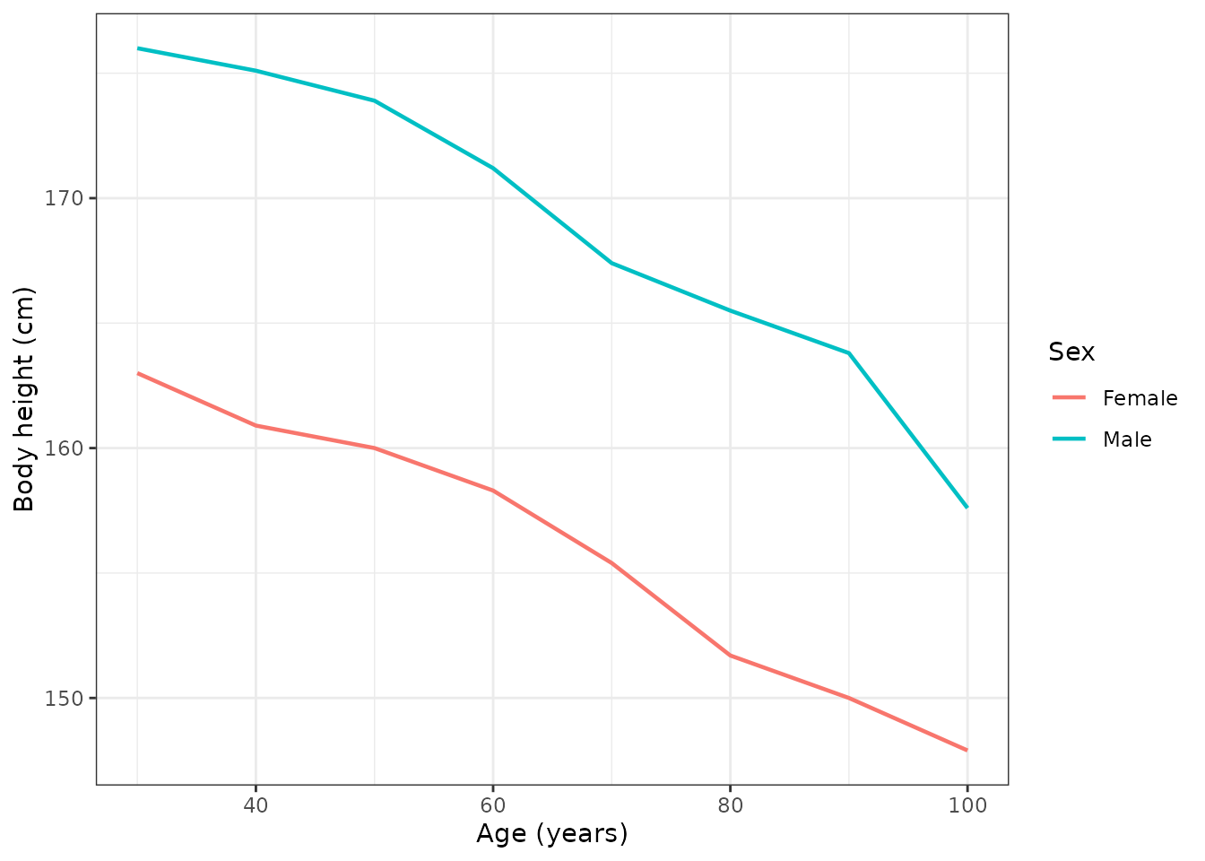
Replicates Figure 3 of Schlender 2016: age-dependent decrease in body height in females and males over 30 to 100 years.
sim_fine |>
  dplyr::select(
    "time", "sex",
    "mass_fat", "mass_muscle", "mass_bone", "mass_skin",
    "mass_liver", "mass_brain", "mass_blood"
  ) |>
  tidyr::pivot_longer(dplyr::starts_with("mass_"), names_to = "tissue", values_to = "g") |>
  dplyr::mutate(tissue = sub("^mass_", "", .data$tissue)) |>
  ggplot2::ggplot(ggplot2::aes(.data$time, .data$g / 1000, colour = .data$tissue)) +
  ggplot2::geom_line(linewidth = 0.7) +
  ggplot2::facet_wrap(~sex) +
  ggplot2::labs(x = "Age (years)", y = "Mass (kg)", colour = "Tissue") +
  ggplot2::theme_bw()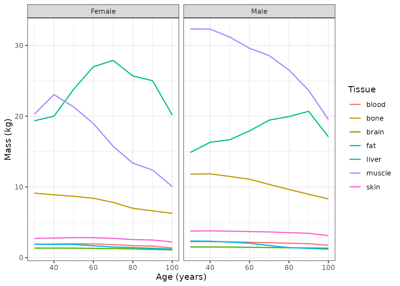
Replicates the 30-100 y portion of Figure 2 of Schlender 2016: distribution of mean organ and tissue weights across the course of aging. Fat rises then falls while muscle and liver decline throughout.
6. The paper’s prose claims, checked against its own tables
Schlender 2016 states a number of quantitative aging rates in the Results narrative. None of them is a model parameter, so none is exercised by the checks above – but each is a claim about the very tables this model encodes, and a transcription error would break the agreement. Converting them into assertions is therefore a genuine gate, and it also surfaces several places where the prose and the tables disagree.
at <- function(v, sex, a) sim_knot[[v]][sim_knot$sex == sex & sim_knot$time == a]
per_decade_pct <- function(v, sex, a0, a1) {
  ((at(v, sex, a1) / at(v, sex, a0))^(10 / (a1 - a0)) - 1) * 100
}

claims <- tibble::tribble(
  ~Claim, ~Source, ~Published, ~Achieved, ~Tol, ~Deviation,
  "Male cardiac index falls 8.30 %/decade in the elderly (60-100 y)",
  "Results 3.1.6", -8.30, per_decade_pct("cardiac_index", "Male", 60, 100), 0.5, FALSE,

  "Splanchnic blood flow is 22.5 % of cardiac output in adults (female, 30 y)",
  "Results 3.1.8", 22.5,
  100 * at("flow_splanchnic", "Female", 30) / at("cardiac_output", "Female", 30), 0.5, FALSE,

  "Splanchnic blood flow falls to 17.5 % of cardiac output in the tenth decade (female, 100 y)",
  "Results 3.1.8", 17.5,
  100 * at("flow_splanchnic", "Female", 100) / at("cardiac_output", "Female", 100), 0.5, FALSE,

  "Male fat mass increases by 0.978 kg/decade, constantly (30-90 y)",
  "Results 3.1.3", 0.978,
  (at("mass_fat", "Male", 90) - at("mass_fat", "Male", 30)) / 1000 / 6, 0.05, FALSE,

  "Female fat mass gains 3.50 kg/decade over the first two decades after menopause (40-60 y)",
  "Results 3.1.3", 3.50,
  (at("mass_fat", "Female", 60) - at("mass_fat", "Female", 40)) / 1000 / 2, 0.05, FALSE,

  "Relative fat mass reaches 45.8 % in female centenarians",
  "Results 3.1.3", 45.8,
  100 * at("mass_fat", "Female", 100) / 1000 / at("bw", "Female", 100), 1.5, FALSE,

  "Relative fat mass reaches 31.5 % in male centenarians",
  "Results 3.1.3", 31.5,
  100 * at("mass_fat", "Male", 100) / 1000 / at("bw", "Male", 100), 1.5, FALSE,

  "Male skeletal muscle is 44 % of body weight in adults (30 y)",
  "Results 3.1.2", 44.0,
  100 * at("mass_muscle", "Male", 30) / 1000 / at("bw", "Male", 30), 1.0, FALSE,

  "Female skeletal muscle falls to 22 % of body weight in centenarians",
  "Results 3.1.2", 22.0,
  100 * at("mass_muscle", "Female", 100) / 1000 / at("bw", "Female", 100), 1.0, FALSE,

  "Male skeletal muscle falls to 34 % of body weight in the extremely old (100 y)",
  "Results 3.1.2", 34.0,
  100 * at("mass_muscle", "Male", 100) / 1000 / at("bw", "Male", 100), 1.5, FALSE,

  "Male body height loses about 3.5 %/decade in the tenth decade",
  "Results 3.1.1", -3.5, per_decade_pct("ht", "Male", 90, 100), 0.5, FALSE,

  "Male liver mass falls 11.4 %/decade after 60 y",
  "Results 3.1.5", -11.4, per_decade_pct("mass_liver", "Male", 60, 100), 1.2, FALSE,

  # ---- Documented deviations: prose vs the paper's own tables ----
  "Female liver mass falls 8.3 %/decade after 40 y",
  "Results 3.1.5", -8.3, per_decade_pct("mass_liver", "Female", 40, 100), 0.5, TRUE,

  "Male liver mass falls 6.1 %/decade up to 60 y",
  "Results 3.1.5", -6.1, per_decade_pct("mass_liver", "Male", 30, 60), 0.5, TRUE,

  "Female cardiac index falls almost linearly by 3.22 %/decade after 30 y",
  "Results 3.1.6", -3.22, per_decade_pct("cardiac_index", "Female", 30, 100), 0.5, TRUE,

  "Male cardiac index falls 1.46 %/decade during early adulthood (30-60 y)",
  "Results 3.1.6", -1.46, per_decade_pct("cardiac_index", "Male", 30, 60), 0.5, TRUE,

  "Female body height loses 4.2 %/decade in nonagenarians",
  "Results 3.1.1", -4.2, per_decade_pct("ht", "Female", 90, 100), 0.5, TRUE,

  "Body weight decline rises to nearly 10 %/decade between 90 and 100 y (female)",
  "Results 3.1.1", -10.0, per_decade_pct("bw", "Female", 90, 100), 1.5, TRUE
) |>
  dplyr::mutate(
    Achieved = round(.data$Achieved, 2),
    Pass = abs(.data$Achieved - .data$Published) <= .data$Tol
  )

# Every non-deviation claim must reproduce. The deviations are kept visible
# in the rendered table rather than having their tolerance widened until
# they disappear.
stopifnot(all(claims$Pass[!claims$Deviation]))
# ... and each recorded deviation must genuinely still be a deviation, so
# this gate goes red if a future edit silently fixes or breaks one.
stopifnot(!any(claims$Pass[claims$Deviation]))

claims |>
  dplyr::select("Claim", "Source", "Published", "Achieved", "Pass", "Deviation") |>
knitr::kable()| Claim | Source | Published | Achieved | Pass | Deviation |
|---|---|---|---|---|---|
| Male cardiac index falls 8.30 %/decade in the elderly (60-100 y) | Results 3.1.6 | -8.300 | -8.10 | TRUE | FALSE |
| Splanchnic blood flow is 22.5 % of cardiac output in adults (female, 30 y) | Results 3.1.8 | 22.500 | 22.56 | TRUE | FALSE |
| Splanchnic blood flow falls to 17.5 % of cardiac output in the tenth decade (female, 100 y) | Results 3.1.8 | 17.500 | 17.43 | TRUE | FALSE |
| Male fat mass increases by 0.978 kg/decade, constantly (30-90 y) | Results 3.1.3 | 0.978 | 0.97 | TRUE | FALSE |
| Female fat mass gains 3.50 kg/decade over the first two decades after menopause (40-60 y) | Results 3.1.3 | 3.500 | 3.50 | TRUE | FALSE |
| Relative fat mass reaches 45.8 % in female centenarians | Results 3.1.3 | 45.800 | 44.63 | TRUE | FALSE |
| Relative fat mass reaches 31.5 % in male centenarians | Results 3.1.3 | 31.500 | 30.72 | TRUE | FALSE |
| Male skeletal muscle is 44 % of body weight in adults (30 y) | Results 3.1.2 | 44.000 | 44.30 | TRUE | FALSE |
| Female skeletal muscle falls to 22 % of body weight in centenarians | Results 3.1.2 | 22.000 | 22.26 | TRUE | FALSE |
| Male skeletal muscle falls to 34 % of body weight in the extremely old (100 y) | Results 3.1.2 | 34.000 | 35.13 | TRUE | FALSE |
| Male body height loses about 3.5 %/decade in the tenth decade | Results 3.1.1 | -3.500 | -3.79 | TRUE | FALSE |
| Male liver mass falls 11.4 %/decade after 60 y | Results 3.1.5 | -11.400 | -12.40 | TRUE | FALSE |
| Female liver mass falls 8.3 %/decade after 40 y | Results 3.1.5 | -8.300 | -7.35 | FALSE | TRUE |
| Male liver mass falls 6.1 %/decade up to 60 y | Results 3.1.5 | -6.100 | -4.69 | FALSE | TRUE |
| Female cardiac index falls almost linearly by 3.22 %/decade after 30 y | Results 3.1.6 | -3.220 | -4.56 | FALSE | TRUE |
| Male cardiac index falls 1.46 %/decade during early adulthood (30-60 y) | Results 3.1.6 | -1.460 | -3.97 | FALSE | TRUE |
| Female body height loses 4.2 %/decade in nonagenarians | Results 3.1.1 | -4.200 | -1.40 | FALSE | TRUE |
| Body weight decline rises to nearly 10 %/decade between 90 and 100 y (female) | Results 3.1.1 | -10.000 | -15.83 | FALSE | TRUE |
Twelve of the eighteen prose claims reproduce from the tables within tolerance. The six that do not are discussed in the Errata below.
Assumptions and deviations
Errata: prose that disagrees with the paper’s own Tables 2 and 3
These are disagreements within the source, not transcription choices. The tables are used, because the tables are what the PBPK model was actually parameterised with (“as used in the elderly PBPK models” – Table 2 caption).
Female body height, “a 4.2 % decrease in body height per decade in female nonagenarians” (Results 3.1.1). Table 2 gives 150.0 cm at 90 y and 147.9 cm at 100 y, a 1.4 % decrease per decade – three-fold smaller. No decade in the female height row reaches 4.2 %; the largest is 2.4 % (70 to 80 y), and even the whole 70-to-100-year span averages 1.6 %/decade. The corresponding male claim (“about 3.5 %” in the tenth decade) does reproduce, at 3.8 %.
Body weight, “rose to nearly 10 % per decade between 90 and 100 years” (Results 3.1.1). Table 2 gives 53.7 to 45.2 kg in females (15.8 %) and 64.9 to 55.6 kg in males (14.3 %). The prose understates the tabulated decline by roughly half.
Female cardiac index, “an almost linear decrease of 3.22 % per decade after the age of 30 years” (Results 3.1.6). The Table 3 female row falls from 3.34 to 2.41 L/min/m^2 over 30 to 100 y, which is 4.56 %/decade, and it is visibly non-linear (essentially flat from 30 to 40 y, then steepening).
Male cardiac index, “1.46 % per decade during early adulthood” (Results 3.1.6). Table 3 gives only 0.31 %/decade from 30 to 40 y and 3.97 %/decade averaged over 30 to 60 y; no window in the tabulated range yields 1.46 %. The companion elderly claim (8.30 %/decade) reproduces almost exactly, at 8.10 %.
Liver mass rates (Results 3.1.5). The female “8.3 %/decade after 40 years” is 7.35 %/decade in Table 2, and the male “6.1 %/decade to the age of 60” is 4.69 %/decade. The male post-60 rate (“11.4 %/decade”) does reproduce, at 12.4 %.
Male body weight peak. The prose says “both sexes showed an increase in body mass up to the age of 55 years”. The female row does peak between the 50- and 60-year knots, but the male row peaks at the 40-year knot (74.4 kg) and declines thereafter. The decade knots cannot resolve an age of 55 in any case.
Two further prose statements are reconciled rather than contradicted, and the window used in the assertion table above reflects the reconciliation:
- “3.50 kg fat mass per decade in the first two decades after menopause” reproduces to three significant figures only over the 40-to-60-year window (3.495 kg/decade), not the 50-to-70-year window a literal reading of “after menopause” suggests (2.04 kg/decade).
- “37 % of body weight in adults” for female skeletal muscle is the value at the 40-year knot (36.4 %), which is where the female muscle row peaks, not at 30 y (33.8 %).
Assumptions made by this extraction
gfr_vmaxis dimensionless. The prose tags the maximal decreasing rate factor as “0.9 mL/min/100 g kidney weight”, carrying over the unit ofF_PMAfrom the preceding sentence. Equation 1 multipliesVmaxby a unitless Hill ratio inside(1 - ...), soVmaxmust be a dimensionless fraction for the equation to be dimensionally consistent – and the resulting curve matches the published Figure 5. It is encoded as a fraction.Body surface area uses the Du Bois equation. Table 3 reports a cardiac index (per m^2 of BSA) but the paper never states which BSA formula it used, so recovering cardiac output requires a choice. Du Bois is used. The choice is not load-bearing: with the Mosteller equation instead, the flow-sum-to-cardiac-output ratios of validation section 3 move by less than 1.5 percentage points and every cell still balances, and
cardiac_indexitself – the published quantity – is unaffected.Flat extrapolation outside 30 to 100 years. Tables 2 and 3 are defined on the 30-to-100-year knots. Below 30 y and above 100 y the model holds the end knot rather than continuing the adjacent decade’s slope, which the paper does not support. Figure 2 of the paper does show organ weights from birth, but those come from the underlying PK-Sim paediatric model, not from this paper’s tables, and are not extracted.
No variability is encoded. The paper assumed a 5 % coefficient of variation on every blood flow rate because “the general lack of perfusion data impeded computation of robust variability” (Results 3.1.8), and made GFR variability depend entirely on kidney-size variability – which the Discussion itself judges “too great”. Neither is a fitted between-subject variance, so neither is encoded as an
eta; this model returns typical values. Organ-mass variability is likewise not reported per organ.The GFR function is evaluated against mean kidney mass. The paper parameterised specific GFR “using the observed GFR values and assuming the mean kidney weight at the respective age” (Results 3.1.10), which is exactly what
gfr <- gfr_specific * mass_kidney / 100does with the Table 2 row.SEXFis an indicator, not a proportion. Every trajectory is published as separate female and male rows and the model blends them linearly bySEXF. Values strictly between 0 and 1 produce a sex-averaged physiology that the paper never reports and that should not be interpreted as a real individual.
Not extracted from this paper
- The morphine and furosemide PBPK drug models (see “What is deliberately not extracted” at the top), including Table 1’s compound cards and Table 5’s predictive-performance statistics.
- Total body water (Figure 4). The paper plots extracellular and total body water as percentages of body weight against age but tabulates no values, and the Discussion notes that no body-water data were available for females above 80 years.
- The per-organ literature review in the Electronic Supplementary Material, which is narrative plus Supplement Table 1 (a list of the contributing studies) and contains no additional parameter values.