Liver lipid metabolism in NAFLD (Rieger 2022)
Source:vignettes/articles/Rieger_2022_liver_lipid_qsp.Rmd
Rieger_2022_liver_lipid_qsp.RmdModel and source
- Citation: Rieger TR, Allen RJ, Musante CJ (2022). A Quantitative Systems Pharmacology Model of Liver Lipid Metabolism for Investigation of Non-Alcoholic Fatty Liver Disease. Front Pharmacol 13:910789. doi:10.3389/fphar.2022.910789. Equations and parameter values are from the authors’ deposited source code (Rieger TR, Allen RJ, Musante CJ (2022) Source Code for a Quantitative Pharmacology Model of Liver Lipid Metabolism, v1.1, doi:10.5281/zenodo.6621096: dxdt.jl, parameters_pluto.csv, util.jl, derived_parameters.jl, main.jl); basal values agree with Supplementary Table S1.
- Article: https://doi.org/10.3389/fphar.2022.910789 (open access, PMC9343875)
- Source code: https://doi.org/10.5281/zenodo.6621096 (Julia, v1.1).
The article describes the model in prose and Figure 1 only; the ODEs are
in
dxdt.jl, the parameter values inparameters_pluto.csv, their derivation inderived_parameters.jl, the liver-fat observable inutil.jland the intervention settings inmain.jl. Supplementary Table S1 prints the same basal values to two significant figures.
Rieger 2022 is a quantitative systems pharmacology (QSP) model of
human hepatocyte lipid metabolism, built to simulate anti-steatotic
therapies in non-alcoholic fatty liver disease (NAFLD). Five ODEs track
cytosolic fatty acids (fa_cy), cytosolic triglyceride
(tg_cy), endoplasmic-reticulum fatty acids and triglyceride
(fa_er, tg_er), and lumped plasma triglyceride
(tg_p). The fluxes are 24-hour averages, so time is in days
and the model has no meal dynamics. Pioglitazone and diet are not given
as doses: each is a step change in one or more of the
scale_* flux multipliers.
Nothing in the model is estimated. The authors derived a basal parameter set from literature fluxes and steady-state constraints, then built virtual patients by sampling the first 14 parameters and keeping those whose steady state matches the joint distribution of liver fat and plasma triglyceride in Kotronen 2007. The packaged model therefore carries no IIV and no residual error. This vignette rebuilds a virtual population the same way and uses it to reproduce Figures 2 to 5.
Population
| Field | Value |
|---|---|
| species | human |
| n_subjects | 1900 |
| disease_state | General adult population spanning normal liver fat, hyperlipidaemia, simple NAFLD and NAFLD with hyperlipidaemia; the NAFLD cohort is the 900 virtual patients with liver fat > 5% (Rieger 2022 Sections 2.4, 3.1). |
| dose_range | No drug PK. Pioglitazone 45 mg QD for 24 weeks (Belfort 2006) is represented as a 27.5% reduction of NEFA uptake; a 26-week diet (Haufe 2013) as -20% chylomicron, -55% DNL and -11% NEFA flux. |
| notes | The 1,900 virtual patients are model constructs selected from 500,000 plausible patients so that steady-state liver fat and plasma TG match a joint log-normal fitted to the digitised individual data of Kotronen 2007 (simultaneous liver fat % and fasting serum TG; TG divided by 0.8 to approximate a 24-h mean). Basal parameters are derived from literature fluxes and steady-state constraints for a 70 kg adult with a 1.5 kg liver eating 2400 kcal/day (35% fat). |
Source trace
| Model element | Source |
|---|---|
ODEs d/dt(fa_cy) to d/dt(tg_p)
|
dxdt.jl (dfa_cy, dtg_cy,
dfa_er, dtg_er, dtg_p); Figure 1
schematic |
Flux expressions (nefa_uptake, er_uptake,
tg_cy_ester, tg_cy_lipo,
tg_er_ester, tg_er_vldl_prod,
tg_p_liver_uptake, tg_p_clear,
chylo_prod, dnl, beta_ox) |
dxdt.jl “Fluxes” block |
| ER lipolysis set to zero |
dxdt.jl (tg_er_lipo = 0.0, with its
footnote on ATGL) |
Cytosolic-FA feedback on NEFA uptake, smooth max with k = 20 and
floor fa_cy_basal / 10
|
dxdt.jl (h(k, x, minx),
denom, nefa_uptake_feedback); Section 2.2 |
| DNL feedback on beta-oxidation |
dxdt.jl (beta_ox_feedback); Section
2.2 |
| Initial conditions = basal concentrations |
main.jl (x0 .= df.TV[23:27]) |
liver_fat (volume %), TG density 0.9 g/mL, MW 772
g/mol, non-TG hepatocyte volume 0.95 x 0.7089 L |
util.jl getLTGprct (vector method);
derived_parameters.jl
|
All 27 ini() values |
parameters_pluto.csv TV column (rows 1-27); Table S1
for rows 1-14 |
Pioglitazone: scale_nefa_uptake 0.725 for 24 weeks |
main.jl (nefa_scalar = 1 - 0.275,
tspan = 24 * 7); Section 2.5 (-28%) |
Diet: scale_chylo 0.8, scale_dnl 0.448,
scale_nefa_uptake 0.89 for 26 weeks |
main.jl; Section 2.6 (-20%, -55%, -11%) |
Sensitivity analysis: scale_dnl,
scale_nefa_uptake, scale_tg_ester from 1 to
0.05; scale_vldl_prod from 1 to 20 |
main.jl (sa_scale,
p_idx_scale, p_scale_inv); Section 2.7 |
| Plausible-patient prior (log-normal, mean TV, SD (HV - LV) / 3.24, parameters 1-14) and steady-state bounds (rows 23-27) |
mh.jl, mh_sim.jl,
parameters_pluto.csv LV / HV columns |
| Target distribution of liver fat and plasma TG |
util.jl joint_tg_dist (176 digitised
Kotronen 2007 points, TG / 0.8) |
| Virtual-patient selection |
select_vps.jl (5-nearest-neighbour density,
acceptance-rejection) |
| Published simulated means (Figures 3, 4, 5) | Digitised by the maintainers from the article figures |
Steady state of the basal parameter set
The basal values were derived so that every pool is at steady state. Solving the typical patient for 1000 days confirms it: no state moves by more than about 1 part in 100,000. The NEFA-uptake feedback is not exactly 1 at basal because its smooth-max denominator is 0.1494 mM rather than 0.15 mM, which accounts for the tiny drift.
ss_typ <- rxSolve(mod, et(c(0, 1000)), returnType = "data.frame")
ss_typ |>
  select(time, fa_cy, tg_cy, fa_er, tg_er, tg_p, liver_fat) |>
knitr::kable(digits = 5)| time | fa_cy | tg_cy | fa_er | tg_er | tg_p | liver_fat |
|---|---|---|---|---|---|---|
| 0 | 0.15 | 58.29016 | 0.15 | 58.29016 | 1.5385 | 4.63762 |
| 1000 | 0.15 | 58.29079 | 0.15 | 58.29083 | 1.5385 | 4.63767 |
drift <- abs(unlist(ss_typ[2, c("fa_cy", "tg_cy", "fa_er", "tg_er", "tg_p")]) /
  unlist(ss_typ[1, c("fa_cy", "tg_cy", "fa_er", "tg_er", "tg_p")]) - 1)
stopifnot(max(drift) < 1e-4)
The typical patient has 4.64% liver fat, so it is just below the 5% NAFLD threshold. Its 24-hour mean plasma triglyceride is 1.54 mM (136 mg/dL).
Fatty-acid mass balance
At steady state the hepatocyte’s fatty-acid inputs (NEFA uptake, DNL
and three FA per TG taken up from plasma) equal its outputs
(beta-oxidation and three FA per TG exported as VLDL). The check below
works directly from the ini() values.
p <- exp(unlist(mod$theta[grepl("^l", names(mod$theta))]))
names(p) <- sub("^l", "", names(p))
vldl <- p[["emax_vldl_prod"]] * p[["tg_er_basal"]] / (p[["ec50_vldl_prod"]] + p[["tg_er_basal"]])
fa_in <- p[["nefa_uptake_flux"]] + p[["dnl_basal_flux"]] +
  3 * p[["kuptake_liver_tg"]] * p[["tg_p_basal"]] * p[["vd_tg_p"]]
fa_out <- p[["kbetaox"]] * p[["fa_cy_basal"]] * p[["vd_cyt"]] + 3 * vldl
c(fa_in_mmol_day = fa_in, fa_out_mmol_day = fa_out, vldl_tg_mmol_day = vldl)
#>   fa_in_mmol_day  fa_out_mmol_day vldl_tg_mmol_day
#>        193.30898        193.30898         23.06995
stopifnot(abs(fa_in / fa_out - 1) < 1e-8)
Virtual population (Figure 2)
The authors drew 500,000 plausible patients with a Metropolis-Hastings independence sampler and kept 1,900 virtual patients by acceptance-rejection. That run is not reproducible here: the file of plausible patients in the code deposit is a Git LFS pointer, not the data. The vignette therefore rebuilds a smaller population with the same ingredients:
- Draw the 14 searched parameters from the authors’ prior. Each is
log-normal with mean equal to its basal value and linear-scale SD
(HV - LV) / 3.24(mh.jl). - Solve each draw to steady state. Discard any draw with a
steady-state concentration outside the bounds in rows 23 to 27 of
parameters_pluto.csv(mh_sim.jl). - Accept each plausible patient with probability proportional to
pdf(target) / local density of plausible patients. The density comes from the median distance to the 5 nearest neighbours in (liver fat %, TG mM) space (select_vps.jl).
In step 1 the authors’ Metropolis-Hastings chain targets prior x target pdf, and their selection step then divides by the local density of those samples. Drawing straight from the prior and dividing by the prior’s density in observable space reaches the same end point: the virtual patients’ observables follow the target distribution.
# parameters_pluto.csv rows 1-14 (searched) and 23-27 (steady-state bounds)
prior_tab <- tibble::tribble(
  ~parameter, ~TV, ~LV, ~HV,
  "klipase_clear", 16.801971423166567, 2.6608094803554985, 66.52023700888748,
  "sens_nefa_uptake", 0.001, 1e-06, 0.1,
  "sens_betaox_dnl", 0.1, 0.010000000000000002, 0.2,
  "kuptake_er", 929.808692197991, 232.45217304949776, 3719.234768791964,
  "kuptake_liver_tg", 0.5734207183549842, 0.14335517958874605, 2.293682873419937,
  "ksynth_cy_tg", 14463.690767524306, 3615.9226918810764, 57854.76307009722,
  "klipo_cy_tg", 0.27914923181321905, 0.06978730795330476, 1.1165969272528762,
  "ksynth_er_tg", 129140.09613860988, 32285.02403465247, 516560.3845544395,
  "kbetaox", 1667.225980228621, 416.80649505715525, 6668.903920914484,
  "emax_vldl_prod", 33.62629534, 8.406573835, 134.50518136,
  "ec50_vldl_prod", 26.67240932642487, 6.668102331606217, 106.68963730569948,
  "chylo_basal_flux", 97.62521588946458, 46.37197754749568, 168.9264896373057,
  "dnl_basal_flux", 9.665448866236932, 0.9665448866236933, 77.32359092989546,
  "nefa_uptake_flux", 171.69402414356475, 85.84701207178237, 686.776096574259
)
state_bounds <- tibble::tribble(
  ~state, ~LV, ~HV,
  "fa_cy", 0.0375, 5.9192307692307695,
  "tg_cy", 3.332536469512164, 2300.2192108409736,
  "fa_er", 0.0375, 5.9192307692307695,
  "tg_er", 3.332536469512164, 2300.2192108409736,
  "tg_p", 0.38860103626943004, 9.715025906735752
)

# Joint log-normal of (liver fat %, 24-h mean TG mM): mean and covariance of
# log() of the 176 digitised Kotronen 2007 points in util.jl, TG divided by 0.8.
target_mu <- c(1.51335179, 0.4790895)
target_cov <- matrix(c(1.60254749, 0.26781155, 0.26781155, 0.30396876), 2)
set.seed(20220719)
n_pp <- 20000
sd_lin <- (prior_tab$HV - prior_tab$LV) / 3.24
mu_log <- log(prior_tab$TV^2 / sqrt(sd_lin^2 + prior_tab$TV^2))
sd_log <- sqrt(log(1 + sd_lin^2 / prior_tab$TV^2))
draws <- vapply(
  seq_len(nrow(prior_tab)),
  function(i) exp(rnorm(n_pp, mu_log[i], sd_log[i])),
  numeric(n_pp)
)
colnames(draws) <- prior_tab$parameter

# Map onto ini() names: everything except the two feedback exponents is
# log-transformed.
log_par <- setdiff(prior_tab$parameter, c("sens_nefa_uptake", "sens_betaox_dnl"))
pp_par <- as.data.frame(draws)
pp_par[log_par] <- log(pp_par[log_par])
names(pp_par)[match(log_par, names(pp_par))] <- paste0("l", log_par)
pp_par$id <- seq_len(n_pp)

# 10,000 days is the end of the authors' steady-state search window.
pp_ss <- rxSolve(
  mod,
  params = pp_par,
  events = data.frame(id = pp_par$id, time = 10000, evid = 0),
  returnType = "data.frame"
)
#> [====|====|====|====|====|====|====|====|====|====] 0:00:08
in_bounds <- Reduce(`&`, lapply(seq_len(nrow(state_bounds)), function(i) {
  x <- pp_ss[[state_bounds$state[i]]]
  !is.na(x) & x >= state_bounds$LV[i] & x <= state_bounds$HV[i]
}))
pp <- pp_ss[in_bounds, ]

dlnorm2 <- function(lf, tg, mu, sigma) {
  z <- cbind(log(lf) - mu[1], log(tg) - mu[2])
  q <- rowSums((z %*% solve(sigma)) * z)
  exp(-q / 2) / (2 * pi * sqrt(det(sigma)) * lf * tg)
}
knn_median_dist <- function(x, k = 5) {
  # Median of the k nearest distances, the point itself included (select_vps.jl).
  vapply(seq_len(nrow(x)), function(i) {
    d <- sqrt((x[, 1] - x[i, 1])^2 + (x[, 2] - x[i, 2])^2)
    stats::median(sort.int(d, partial = seq_len(k))[seq_len(k)])
  }, numeric(1))
}

obs <- cbind(pp$liver_fat, pp$tg_p)
pdf_target <- dlnorm2(pp$liver_fat, pp$tg_p, target_mu, target_cov)
rho <- 5 / (pi * knn_median_dist(obs)^2)
p_incl <- pdf_target / rho
selected <- runif(nrow(pp)) < p_incl / max(p_incl)
vp <- pp[selected, ]
vp$nafld <- vp$liver_fat > 5

c(
  plausible_in_bounds = nrow(pp),
  virtual_patients = nrow(vp),
  nafld = sum(vp$nafld)
)
#> plausible_in_bounds    virtual_patients               nafld
#>                5279                 477                 228
Of the virtual patients, 48% have liver fat above 5%. The paper had 900 of 1,900 (47%), and the target distribution implies 47%. The table compares the log-scale moments of the rebuilt population with the target.
vp_moments <- tibble::tibble(
  Statistic = c("mean log liver fat", "SD log liver fat", "mean log TG", "SD log TG", "correlation"),
  Target = c(target_mu[1], sqrt(target_cov[1, 1]), target_mu[2], sqrt(target_cov[2, 2]),
             target_cov[1, 2] / sqrt(target_cov[1, 1] * target_cov[2, 2])),
  `Virtual population` = c(
    mean(log(vp$liver_fat)), sd(log(vp$liver_fat)),
    mean(log(vp$tg_p)), sd(log(vp$tg_p)),
    cor(log(vp$liver_fat), log(vp$tg_p))
  )
)
knitr::kable(vp_moments, digits = 3)| Statistic | Target | Virtual population |
|---|---|---|
| mean log liver fat | 1.513 | 1.534 |
| SD log liver fat | 1.266 | 1.123 |
| mean log TG | 0.479 | 0.479 |
| SD log TG | 0.551 | 0.530 |
| correlation | 0.384 | 0.326 |
stopifnot(
  abs(mean(log(vp$liver_fat)) - target_mu[1]) < 0.3,
  abs(mean(log(vp$tg_p)) - target_mu[2]) < 0.15,
  abs(mean(vp$nafld) - 0.47) < 0.1
)
theta <- seq(0, 2 * pi, length.out = 200)
ev <- eigen(target_cov)
ellipse <- t(target_mu + ev$vectors %*% (sqrt(ev$values * qchisq(0.95, 2)) * rbind(cos(theta), sin(theta))))
ggplot(vp, aes(log(liver_fat), log(tg_p), colour = nafld)) +
  geom_point(alpha = 0.6, size = 1) +
  geom_path(
    data = data.frame(x = ellipse[, 1], y = ellipse[, 2]),
    aes(x, y), inherit.aes = FALSE, colour = "black", linewidth = 0.8
  ) +
  scale_colour_manual(values = c(`FALSE` = "steelblue", `TRUE` = "firebrick"),
                      labels = c("liver fat <= 5%", "NAFLD (> 5%)"), name = NULL) +
  labs(x = "log(liver fat, %)", y = "log(24-h mean plasma TG, mM)",
       caption = "Replicates Figure 2 of Rieger 2022. Ellipse: 95% region of the target distribution.") +
  theme_bw()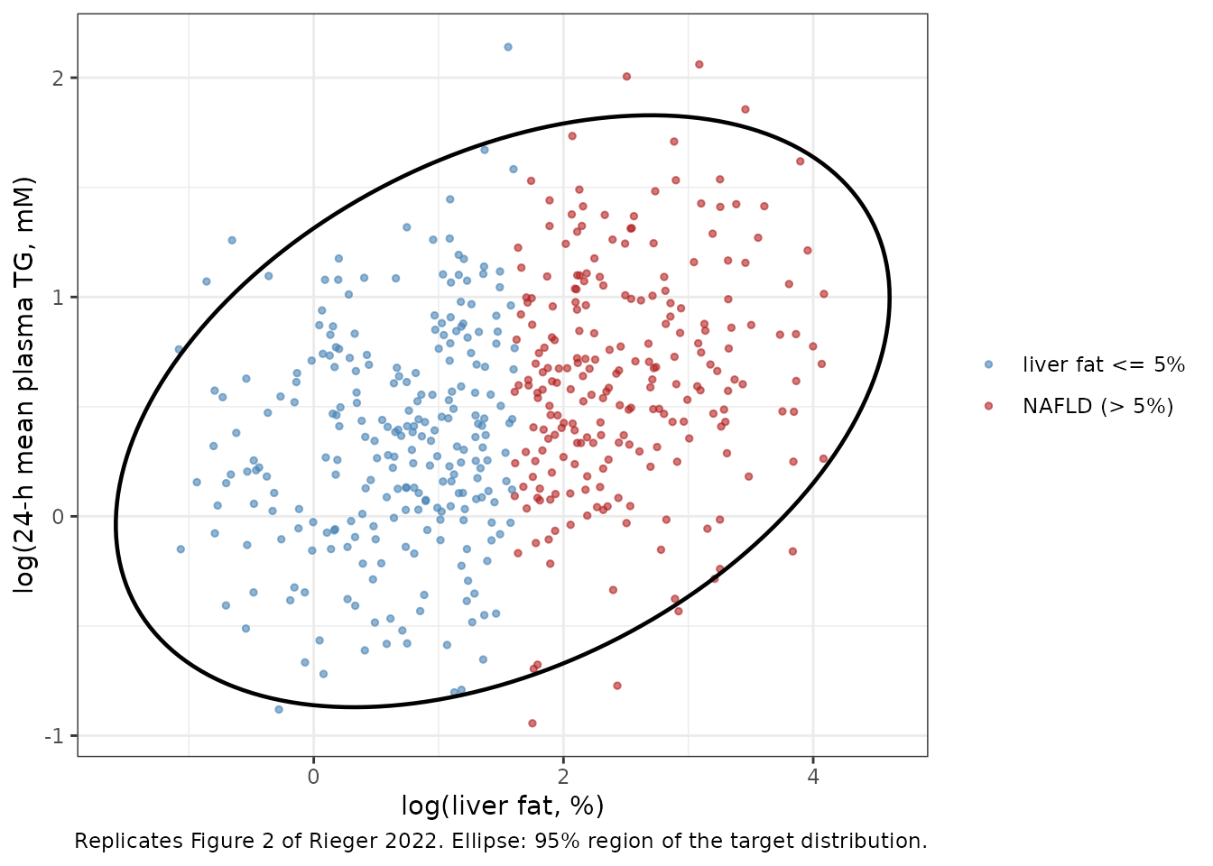
Pioglitazone and diet (Figures 3 and 4)
The paper validates the model on two interventions, both simulated in the NAFLD virtual patients with no refitting:
-
Pioglitazone 45 mg QD for 24 weeks (Belfort 2006):
NEFA release from adipose falls by 27.5%
(
scale_nefa_uptake = 0.725). -
Diet for 26 weeks (Haufe 2013): chylomicron input
-20%, DNL -55.2%, NEFA flux -11% (
scale_chylo = 0.8,scale_dnl = 0.448,scale_nefa_uptake = 0.89).
Each virtual patient runs to its steady state over 10,000 days at
scale_* = 1. The multipliers then step to their treatment
values as time-varying data columns, which override the
ini() values from that row onward. At most 200 NAFLD
virtual patients are used in each arm.
nafld_vp <- vp |>
  filter(nafld) |>
  slice_head(n = 200) |>
  select(id)
nafld_par <- pp_par[match(nafld_vp$id, pp_par$id), ]
nafld_par$id <- seq_len(nrow(nafld_par))

t_run_in <- 10000
run_intervention <- function(scales, weeks, par = nafld_par) {
  ev <- tidyr::expand_grid(id = par$id, time = c(0, t_run_in, t_run_in + 7 * weeks))
  ev$evid <- 0
  for (nm in c("scale_chylo", "scale_dnl", "scale_nefa_uptake", "scale_tg_ester", "scale_vldl_prod")) {
    value <- if (nm %in% names(scales)) scales[[nm]] else 1
    ev[[nm]] <- ifelse(ev$time >= t_run_in, value, 1)
  }
  sim <- rxSolve(mod, params = par, events = ev, returnType = "data.frame")
  # rxSolve() drops the id column for a single subject.
  if (!"id" %in% names(sim)) sim$id <- 1L
  sim |>
    filter(time >= t_run_in) |>
    mutate(phase = ifelse(time == t_run_in, "baseline", "end")) |>
    select(id, phase, liver_fat, tg_cy, tg_er) |>
    pivot_wider(names_from = phase, values_from = c(liver_fat, tg_cy, tg_er)) |>
    mutate(pct_change = 100 * (liver_fat_end / liver_fat_baseline - 1))
}

pio <- run_intervention(c(scale_nefa_uptake = 0.725), weeks = 24)
diet <- run_intervention(c(scale_chylo = 0.8, scale_dnl = 0.448, scale_nefa_uptake = 0.89), weeks = 26)
In main.jl, the code that produced Figures 3 to 5
computes baseline liver fat with getLTGprct’s vector
method, which uses a non-TG hepatocyte volume of 0.95 x 0.7089 = 0.673
L. It computes the end-of-treatment value with the matrix method, which
uses vd_cyt + vd_er = 0.655 L. The packaged
liver_fat output uses 0.673 L at both time points. The “as
coded” column recomputes the end value the way the figure code does, to
show how far the mismatch moves the published means.
as_coded_end <- function(d, vd_cyt = 0.4962299999999999, vd_er = 0.15879359999999998) {
  v <- (d$tg_cy_end * vd_cyt + d$tg_er_end * vd_er) * 772 / 1000 / 900
  100 * v / (v + vd_cyt + vd_er)
}
summarise_arm <- function(d) {
  coded <- 100 * (as_coded_end(d) / d$liver_fat_baseline - 1)
  c(mean = mean(d$pct_change), sd = stats::sd(d$pct_change), mean_as_coded = mean(coded))
}
fig34 <- tibble::tibble(
  Intervention = c("Pioglitazone, 24 weeks", "Diet, 26 weeks"),
  `Observed mean (SD)` = c("-54 (5.4)", "-44.6 (19.3)"),
  `Published simulation mean (SD)` = c("-50.4 (12.0)", "-43.5 (13.0)"),
  `This vignette, mean` = c(summarise_arm(pio)[["mean"]], summarise_arm(diet)[["mean"]]),
  `This vignette, SD` = c(summarise_arm(pio)[["sd"]], summarise_arm(diet)[["sd"]]),
  `This vignette, mean as coded` = c(summarise_arm(pio)[["mean_as_coded"]], summarise_arm(diet)[["mean_as_coded"]])
)
knitr::kable(fig34, digits = 1)| Intervention | Observed mean (SD) | Published simulation mean (SD) | This vignette, mean | This vignette, SD | This vignette, mean as coded |
|---|---|---|---|---|---|
| Pioglitazone, 24 weeks | -54 (5.4) | -50.4 (12.0) | -51.2 | 11.1 | -49.9 |
| Diet, 26 weeks | -44.6 (19.3) | -43.5 (13.0) | -44.2 | 12.1 | -42.8 |
The observed values are Belfort 2006 and Haufe 2013 as given in
main.jl (data_pio_mean,
data_diet_mean and their SDs). The published simulation
means and SDs were digitised by the maintainers from the error bars in
Figures 3 and 4. Digitising the observed bars in the same figures
returns -54.0 (5.4) and -44.6 (19.3), which confirms the
digitisation.
bind_rows(
  mutate(pio, Intervention = "Pioglitazone (Figure 3)"),
  mutate(diet, Intervention = "Diet (Figure 4)")
) |>
  ggplot(aes(Intervention, pct_change)) +
  geom_violin(fill = "darkorange", alpha = 0.5) +
  geom_point(
    data = data.frame(
      Intervention = c("Pioglitazone (Figure 3)", "Diet (Figure 4)"),
      pct_change = c(-54, -44.6)
    ),
    colour = "purple", size = 3
  ) +
  geom_point(
    data = data.frame(
      Intervention = c("Pioglitazone (Figure 3)", "Diet (Figure 4)"),
      pct_change = c(-50.4, -43.5)
    ),
    colour = "black", shape = 4, size = 3
  ) +
  labs(
    y = "Change in liver fat (%)", x = NULL,
    caption = paste(
      "Replicates Figures 3, 4 and S1 of Rieger 2022. Violins: NAFLD virtual patients;",
      "purple: observed mean; cross: published simulated mean."
    )
  ) +
  coord_cartesian(ylim = c(-100, 0)) +
  theme_bw()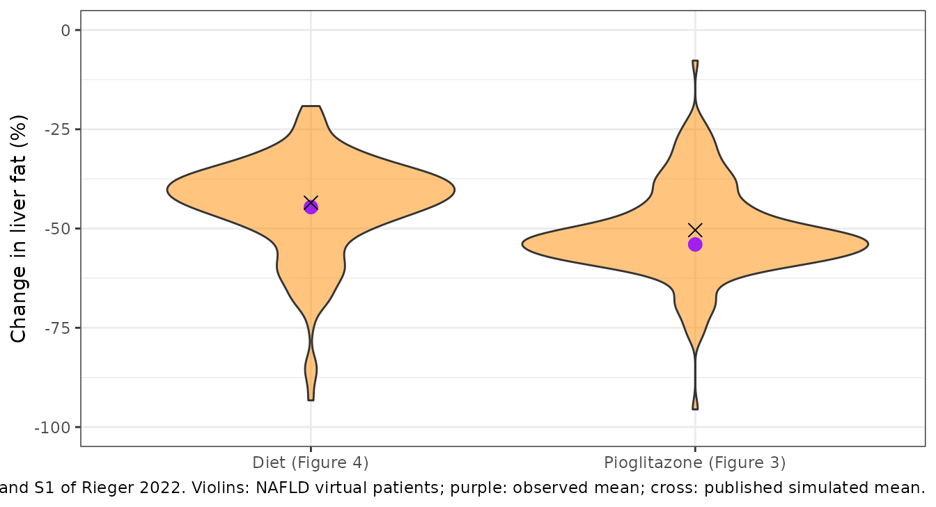
Sensitivity analysis (Figure 5)
Each of four fluxes is held at a constant inhibition for 26 weeks:
DNL, NEFA uptake and cytosolic esterification are scaled by
1 - inhibition. VLDL export is instead activated by
1 / (1 - inhibition), so 95% on the x-axis means 20-fold
activation. The curves are means over the NAFLD virtual patients.
inhibition <- c(0, 10, 25, 50, 75, 90, 95)
sa_targets <- c(DNL = "scale_dnl", `NEFA uptake` = "scale_nefa_uptake",
                Esterification = "scale_tg_ester", `VLDL synthesis (activated)` = "scale_vldl_prod")
sa <- bind_rows(lapply(names(sa_targets), function(lbl) {
  bind_rows(lapply(inhibition, function(inh) {
    value <- if (lbl == "VLDL synthesis (activated)") 1 / (1 - inh / 100) else 1 - inh / 100
    d <- run_intervention(stats::setNames(value, sa_targets[[lbl]]), weeks = 26)
    tibble::tibble(
      intervention = lbl, inhibition = inh,
      mean_pct_change = mean(d$pct_change),
      mean_as_coded = mean(100 * (as_coded_end(d) / d$liver_fat_baseline - 1))
    )
  }))
}))

ggplot(sa, aes(inhibition, mean_pct_change, colour = intervention)) +
  geom_line(linewidth = 1) +
  geom_point() +
  coord_cartesian(ylim = c(-100, 0)) +
  labs(x = "Mean inhibition (%)", y = "Change in liver fat (%)", colour = NULL,
       caption = "Replicates Figure 5 of Rieger 2022 (NAFLD virtual-patient mean).") +
  theme_bw()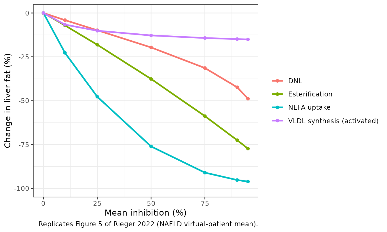
The maintainers digitised the Figure 5 curves at 25, 50, 75 and 90% inhibition (colour-matched pixel columns). The published curves were computed with the mismatched end-of-treatment hepatocyte volume described above. For small changes the mismatch is most visible: it makes the VLDL curve about 2.5 points less negative. So the comparison is made on the “as coded” column.
fig5_pub <- tibble::tribble(
  ~intervention, ~inhibition, ~published,
  "DNL", 25, -8.2, "DNL", 50, -18.4, "DNL", 75, -30.7, "DNL", 90, -41.9,
  "NEFA uptake", 25, -46.8, "NEFA uptake", 50, -75.9, "NEFA uptake", 75, -91.1, "NEFA uptake", 90, -95.4,
  "Esterification", 25, -16.3, "Esterification", 50, -36.5, "Esterification", 75, -58.7, "Esterification", 90, -72.7,
  "VLDL synthesis (activated)", 25, -7.8, "VLDL synthesis (activated)", 50, -10.2,
  "VLDL synthesis (activated)", 75, -11.6, "VLDL synthesis (activated)", 90, -12.2
)
fig5_cmp <- inner_join(fig5_pub, sa, by = c("intervention", "inhibition")) |>
  mutate(difference = mean_as_coded - published)
fig5_cmp |>
  rename(
    Intervention = intervention, `Inhibition (%)` = inhibition,
    `Published (digitised)` = published, `This vignette` = mean_pct_change,
    `This vignette, as coded` = mean_as_coded, `Difference, as coded` = difference
  ) |>
knitr::kable(digits = 1)| Intervention | Inhibition (%) | Published (digitised) | This vignette | This vignette, as coded | Difference, as coded |
|---|---|---|---|---|---|
| DNL | 25 | -8.2 | -9.8 | -7.7 | 0.5 |
| DNL | 50 | -18.4 | -19.6 | -17.7 | 0.7 |
| DNL | 75 | -30.7 | -31.4 | -29.7 | 1.0 |
| DNL | 90 | -41.9 | -42.3 | -40.9 | 1.0 |
| NEFA uptake | 25 | -46.8 | -47.7 | -46.4 | 0.4 |
| NEFA uptake | 50 | -75.9 | -76.0 | -75.4 | 0.5 |
| NEFA uptake | 75 | -91.1 | -91.0 | -90.7 | 0.4 |
| NEFA uptake | 90 | -95.4 | -95.2 | -95.1 | 0.3 |
| Esterification | 25 | -16.3 | -18.1 | -16.1 | 0.2 |
| Esterification | 50 | -36.5 | -37.6 | -36.0 | 0.5 |
| Esterification | 75 | -58.7 | -58.8 | -57.7 | 1.0 |
| Esterification | 90 | -72.7 | -72.5 | -71.8 | 0.9 |
| VLDL synthesis (activated) | 25 | -7.8 | -10.1 | -8.0 | -0.2 |
| VLDL synthesis (activated) | 50 | -10.2 | -12.8 | -10.7 | -0.5 |
| VLDL synthesis (activated) | 75 | -11.6 | -14.3 | -12.2 | -0.6 |
| VLDL synthesis (activated) | 90 | -12.2 | -14.9 | -12.8 | -0.6 |
# The ranking the paper reports (NEFA uptake > esterification > DNL > VLDL) at
# 90% inhibition, and agreement with the digitised curves. The bounds are on the
# centre and a robust quantile because the virtual population is a random draw.
rank_at <- function(inh) {
  x <- sa[sa$inhibition == inh, ]
  x$intervention[order(x$mean_pct_change)]
}
stopifnot(
  identical(rank_at(90), c("NEFA uptake", "Esterification", "DNL", "VLDL synthesis (activated)")),
  abs(median(fig5_cmp$difference)) < 3,
  quantile(abs(fig5_cmp$difference), 0.9) < 5
)
Typical patient
For reference, the same interventions applied to the typical (basal) parameter set give the following responses. The typical patient sits just below the NAFLD threshold.
typ_par <- data.frame(id = 1)
typ <- bind_rows(
  run_intervention(c(scale_nefa_uptake = 0.725), 24, typ_par) |> mutate(Intervention = "Pioglitazone, 24 weeks"),
  run_intervention(c(scale_chylo = 0.8, scale_dnl = 0.448, scale_nefa_uptake = 0.89), 26, typ_par) |>
    mutate(Intervention = "Diet, 26 weeks")
)
typ |>
  select(Intervention, liver_fat_baseline, liver_fat_end, pct_change) |>
  rename(
    `Baseline liver fat (%)` = liver_fat_baseline, `End liver fat (%)` = liver_fat_end,
    `Change (%)` = pct_change
  ) |>
knitr::kable(digits = 2)| Intervention | Baseline liver fat (%) | End liver fat (%) | Change (%) |
|---|---|---|---|
| Pioglitazone, 24 weeks | 4.64 | 2.10 | -54.62 |
| Diet, 26 weeks | 4.64 | 2.64 | -43.03 |
Assumptions and deviations
- Source of the equations. The article prints no equations. The model is transcribed from the authors’ Zenodo code deposit (v1.1, doi:10.5281/zenodo.6621096), which the article cites as the full specification. Every value matches Supplementary Table S1 to the two significant figures printed there.
-
Pioglitazone effect size. Section 2.5 reports a
-28% change in NEFA uptake. The code uses
1 - 0.275, and that value is packaged as the intervention setting. Section 3.2 attributes the NEFA reduction to “the Haufe et al. (2013) study”; the Methods and the code make clear it comes from Belfort 2006. -
Diet DNL reduction. Section 2.6 reports -55%; the
code uses
scale_dnl = 0.448(-55.2%), which is used here. -
Liver-fat observable. The figure code uses two
different non-TG hepatocyte volumes, 0.673 L at baseline and 0.655 L at
the end of treatment. The packaged
liver_fatoutput uses 0.673 L throughout, the value the authors used to select virtual patients (mh_sim.jl,GetObs). The “as coded” column above shows the effect of the mismatch on the published means. -
Virtual population. The authors’ 500,000 plausible
patients are not in the deposit (
save_pp.jld2is a Git LFS pointer). The vignette rebuilds a smaller population from 20,000 prior draws by direct acceptance-rejection rather than a Metropolis-Hastings chain. The selection weights and the target distribution follow the source code, so the rebuilt population matches the target moments but is not the published one. -
Interventions as data columns. The authors change
the parameter vector and restart the ODE from each patient’s steady
state. Here the
scale_*multipliers are passed as time-varying columns in the event table after a 10,000-day run-in, which is equivalent. -
No IIV or residual error. Variability lives
entirely in the virtual population. The packaged model is the
deterministic basal patient, and its
ini()values are all fixed.