Two-compartment zero-order-absorption Michaelis-Menten methodology template (Ibrahim 2019) • nlmixr2lib

Model and source

Citation: Ibrahim MMA, Ueckert S, Freiberga S, Kjellsson MC, Karlsson MO. Model-Based Conditional Weighted Residuals Analysis for Structural Model Assessment. AAPS J. 2019;21(3):34. doi:10.1208/s12248-019-0305-2. PMCID PMC6394649. Structure and all six parameter values transcribed from Supplementary Material 1 (12248_2019_305_MOESM1_ESM.docx), section ‘Simple PK example’, Table 1 ‘Simulation specifications and dOFVBias’.
Article: https://doi.org/10.1208/s12248-019-0305-2

Ibrahim 2019 is a methodology paper. Its own product is a diagnostic: conditional weighted residuals (CWRES) from a fitted nonlinear mixed-effects model are themselves modelled, first by a base model that estimates the mean and variance of the CWRES distribution and then by an extended model that estimates a separate mean for each of N bins of an independent variable. The bin-specific means form a CWRES bias vector, and inverting the FOCE covariance equation converts that vector into a bias in conditional predictions. The method now ships in PsN as part of the qa tool (from version 4.8.1).

That diagnostic is a regression on residuals, not a pharmacokinetic model, and is not encoded in nlmixr2lib. Neither are the two demonstration vehicles of the main text – the integrated glucose-insulin (IGI) model of Silber 2007 and the integrated minimal model (IMM) of Largajolli 2013 – because this paper reports no parameter values for either; they are separate primary sources.

What is packaged here is the paper’s own generative simulation model from Supplementary Material 1, section “Simple PK example”: a two-compartment model with zero-order absorption and Michaelis-Menten elimination, from which the authors simulated 100 subjects. Table 1 of that supplement lists all six structural constants, which makes this a fully-valued author-invented toy model of the same class as Beal_2001_iv1cmt_bql and the Schoning_2026_oral1cmt_* family – and it is filed alongside them under inst/modeldb/pharmacokinetics/ for the same reason: there is no drug.

mod <- readModelDb("Ibrahim_2019_oral2cmt_zeroorder_mm")()
mod
#>  ── rxode2-based free-form 2-cmt ODE model ────────────────────────────────────── 
#>  ── Initalization: ──  
#> Fixed Effects ($theta): 
#>      lvc      lvp       lq    lvmax      lkm      lr1    addSd 
#> 1.420696 1.945910 1.175573 2.220290 2.793616 2.330200 0.000000 
#> 
#> States ($state or $stateDf): 
#>   Compartment Number Compartment Name
#> 1                  1          central
#> 2                  2      peripheral1
#>  ── Model (Normalized Syntax): ── 
#> function() {
#>     compartmentData <- list(central = list(analyte = "hypothetical drug", 
#>         units = NA_character_, specimen = "not applicable", verified = FALSE), 
#>         peripheral1 = list(analyte = "hypothetical drug", units = NA_character_, 
#>             specimen = "not applicable", verified = FALSE))
#>     covariateData <- list()
#>     description <- "Methodology reference. Ground-truth (data-generating) two-compartment population PK model with ZERO-ORDER absorption and Michaelis-Menten elimination for a HYPOTHETICAL drug, taken from the 'Simple PK example' in the supplementary material of Ibrahim 2019, the paper that introduces model-based conditional weighted residuals (CWRES) analysis for structural model assessment. There is no real molecule and no real patients: the authors DEFINED these six structural parameters, simulated a data set of 100 subjects from them, and then fitted that data set with both the true model and a deliberately misspecified variant (first-order instead of zero-order absorption) so that their CWRES-bias diagnostic could be shown to recover a known prediction bias. Every value here is therefore an author-chosen simulation constant, not an estimate, and all are encoded with fixed(). The source reports no units, no dose, no inter-individual variability magnitudes and no residual-error magnitude; the model is consequently typical-value-only and its units are placeholders. See the vignette Errata for the full list of gaps and the one interpretive call (ka0 read as a zero-order input RATE, per its printed row label)."
#>     population <- list(species = "None (methodology paper; simulation-only toy model with no drug, no patients and no fitted estimates).", 
#>         n_subjects = 100L, n_studies = 1L, disease_state = "N/A (Monte Carlo simulation study demonstrating a model-diagnostic method; not a fit of any real molecule).", 
#>         dose_range = "Not reported. The supplement states only that a data set of 100 subjects was simulated; it gives no dose amount, no dosing route beyond 'zero order absorption', and no sampling schedule.", 
#>         regions = "N/A", scope_note = "Filed under inst/modeldb/pharmacokinetics/ (not specificDrugs/) because there is no drug: the model is an author-invented hypothetical used to demonstrate a diagnostic method. This mirrors the packaging of Beal_2001_iv1cmt_bql.R and the Schoning_2026_oral1cmt_* family. The paper's own product is a CWRES-bias regression (a residual post-processing diagnostic, now shipped in PsN's qa tool from version 4.8.1), which is not a pharmacokinetic model and is not encoded here. The two integrated glucose-insulin models the main text uses as demonstration vehicles (the IGI model of Silber 2007, doi:10.1177/0091270007304457, and the integrated minimal model of Largajolli 2013, PAGE 22 Abstract 2762) are cited backbones whose parameter values appear nowhere in this paper or its supplement; they are separate primary sources, not layers of this extraction.", 
#>         notes = "Supplementary Material 1, 'Simple PK example': 'In this example we used a two-compartment PK model with zero order absorption and Michaelis-Menten elimination to simulate a dataset of 100 subjects. The simulated data set was then used to fit two models: a true model (same as the simulation model) and a misspecified model that is the same as the simulation model except for using 1st order absorption process instead of the true zero order absorption process.' Table 1 of that supplement reports dOFVBias = -165.8 for the misspecified fit and lists the six 'Simulated parameters' encoded below, with the footnote 'Vc volume of central compartment, Vp volume of peripheral compartment, ka0 zero order absorption rate, Q intercompartmental clearance, KM and VMAX Michaelis-Menten elimination parameters.' The misspecified companion fit is NOT encoded as a sibling model file because the supplement publishes no parameter values for it; see the vignette Errata.")
#>     reference <- "Ibrahim MMA, Ueckert S, Freiberga S, Kjellsson MC, Karlsson MO. Model-Based Conditional Weighted Residuals Analysis for Structural Model Assessment. AAPS J. 2019;21(3):34. doi:10.1208/s12248-019-0305-2. PMCID PMC6394649. Structure and all six parameter values transcribed from Supplementary Material 1 (12248_2019_305_MOESM1_ESM.docx), section 'Simple PK example', Table 1 'Simulation specifications and dOFVBias'."
#>     units <- list(time = "time_unit", dosing = "dose_unit", concentration = "dose_unit/volume_unit")
#>     vignette <- "Ibrahim_2019_oral2cmt_zeroorder_mm"
#>     ini({
#>         lvc <- fix(1.42069578783722)
#>         label("Central volume of distribution Vc (volume_unit)")
#>         lvp <- fix(1.94591014905531)
#>         label("Peripheral volume of distribution Vp (volume_unit)")
#>         lq <- fix(1.17557332980424)
#>         label("Intercompartmental clearance Q (volume_unit/time_unit)")
#>         lvmax <- fix(2.22028985026722)
#>         label("Michaelis-Menten maximum elimination rate VMAX (dose_unit/time_unit)")
#>         lkm <- fix(2.79361608943186)
#>         label("Michaelis-Menten constant KM (dose_unit/volume_unit)")
#>         lr1 <- fix(2.33020026002702)
#>         label("Zero-order input rate ka0 into the central compartment (dose_unit/time_unit)")
#>         addSd <- fix(0, 0)
#>         label("Additive residual SD; magnitude not reported by the source")
#>     })
#>     model({
#>         vc <- exp(lvc)
#>         vp <- exp(lvp)
#>         q <- exp(lq)
#>         vmax <- exp(lvmax)
#>         km <- exp(lkm)
#>         r1 <- exp(lr1)
#>         Cc <- central/vc
#>         Cp <- peripheral1/vp
#>         rate(central) <- r1
#>         d/dt(central) <- -q * (Cc - Cp) - vmax * Cc/(km + Cc)
#>         d/dt(peripheral1) <- q * (Cc - Cp)
#>         Cc ~ add(addSd)
#>     })
#> }

Population

There is no population. The supplement states only that a data set of 100 subjects was simulated from the model below; it names no molecule, no subjects, no indication and no study. The full metadata list is available programmatically:

str(readModelDb("Ibrahim_2019_oral2cmt_zeroorder_mm")()$meta$population)
#> List of 8
#>  $ species      : chr "None (methodology paper; simulation-only toy model with no drug, no patients and no fitted estimates)."
#>  $ n_subjects   : int 100
#>  $ n_studies    : int 1
#>  $ disease_state: chr "N/A (Monte Carlo simulation study demonstrating a model-diagnostic method; not a fit of any real molecule)."
#>  $ dose_range   : chr "Not reported. The supplement states only that a data set of 100 subjects was simulated; it gives no dose amount"| __truncated__
#>  $ regions      : chr "N/A"
#>  $ scope_note   : chr "Filed under inst/modeldb/pharmacokinetics/ (not specificDrugs/) because there is no drug: the model is an autho"| __truncated__
#>  $ notes        : chr "Supplementary Material 1, 'Simple PK example': 'In this example we used a two-compartment PK model with zero or"| __truncated__

Source trace

Every value in ini() comes from one place: Supplementary Material 1 (12248_2019_305_MOESM1_ESM.docx), section “Simple PK example”, Table 1 “Simulation specifications and dOFVBias”, column “Simulated parameters”. The table’s own footnote supplies the parameter glossary quoted below.

Item	Source location
Two-compartment disposition	Suppl. 1, ‘Simple PK example’, sentence 1
Zero-order absorption	Suppl. 1, ‘Simple PK example’, sentence 1
Michaelis-Menten elimination	Suppl. 1, ‘Simple PK example’, sentence 1
lvc	Suppl. 1, Table 1: Vc = 4.14
lvp	Suppl. 1, Table 1: VP = 7
lq	Suppl. 1, Table 1: Q = 3.24 (‘Q intercompartmental clearance’)
lr1	Suppl. 1, Table 1: ka0 = 10.28 (‘ka0 zero order absorption rate’)
lkm	Suppl. 1, Table 1: KM = 16.34
lvmax	Suppl. 1, Table 1: VMAX = 9.21
addSd	NOT REPORTED anywhere in the paper or supplement; set to fixed(0)
IIV (all parameters)	NOT REPORTED anywhere in the paper or supplement; omitted

Simulation design

The supplement reports no dose, no units and no sampling schedule, so none of those can be traced to the source. The design below is therefore a demonstration of the encoded structure, not a replication of the authors’ simulation: three single doses are given on a ladder chosen to straddle KM, so that the Michaelis-Menten arm is exercised from the near-linear regime into saturation. Because the model carries no IIV and no residual error, every subject within an arm would be identical; one profile per arm is simulated.

Under the encoding, ka0 is an input rate, so the zero-order input lasts amt / ka0 time units and differs by arm.

r1 <- exp(mod$theta[["lr1"]])
km <- exp(mod$theta[["lkm"]])
vc <- exp(mod$theta[["lvc"]])

doses <- c(low = 10, mid = 50, high = 200)
t_inf <- doses / r1

events <-
  dplyr::bind_rows(lapply(seq_along(doses), function(i) {
    e <- rxode2::et(amt = doses[[i]], rate = -1, cmt = "central")
    e <- rxode2::et(e, seq(0, 48, by = 0.05))
    d <- as.data.frame(e)
    d$id <- i
    d$treatment <- names(doses)[i]
    d
  }))

knitr::kable(
  data.frame(
    treatment = names(doses),
    `Dose (dose_unit)` = as.numeric(doses),
    `Zero-order input duration = amt / ka0 (time_unit)` = round(as.numeric(t_inf), 3),
    check.names = FALSE
  )
)

treatment	Dose (dose_unit)	Zero-order input duration = amt / ka0 (time_unit)
low	10	0.973
mid	50	4.864
high	200	19.455

sim <- rxode2::rxSolve(mod, events, returnType = "data.frame")
#> Warning: multi-subject simulation without without 'omega'
sim$treatment <- events$treatment[match(sim$id, events$id)]

ggplot2::ggplot(sim, ggplot2::aes(time, Cc, colour = treatment)) +
  ggplot2::geom_line(linewidth = 0.8) +
  ggplot2::geom_vline(
    data = data.frame(treatment = names(doses), t_inf = as.numeric(t_inf)),
    ggplot2::aes(xintercept = t_inf, colour = treatment),
    linetype = "dashed"
  ) +
  ggplot2::labs(
    x = "Time (time_unit)", y = "Cc (dose_unit/volume_unit)",
    colour = "Dose arm",
    title = "Zero-order input with Michaelis-Menten elimination",
    subtitle = "Dashed lines mark the end of the zero-order input, amt / ka0"
  ) +
  ggplot2::theme_bw()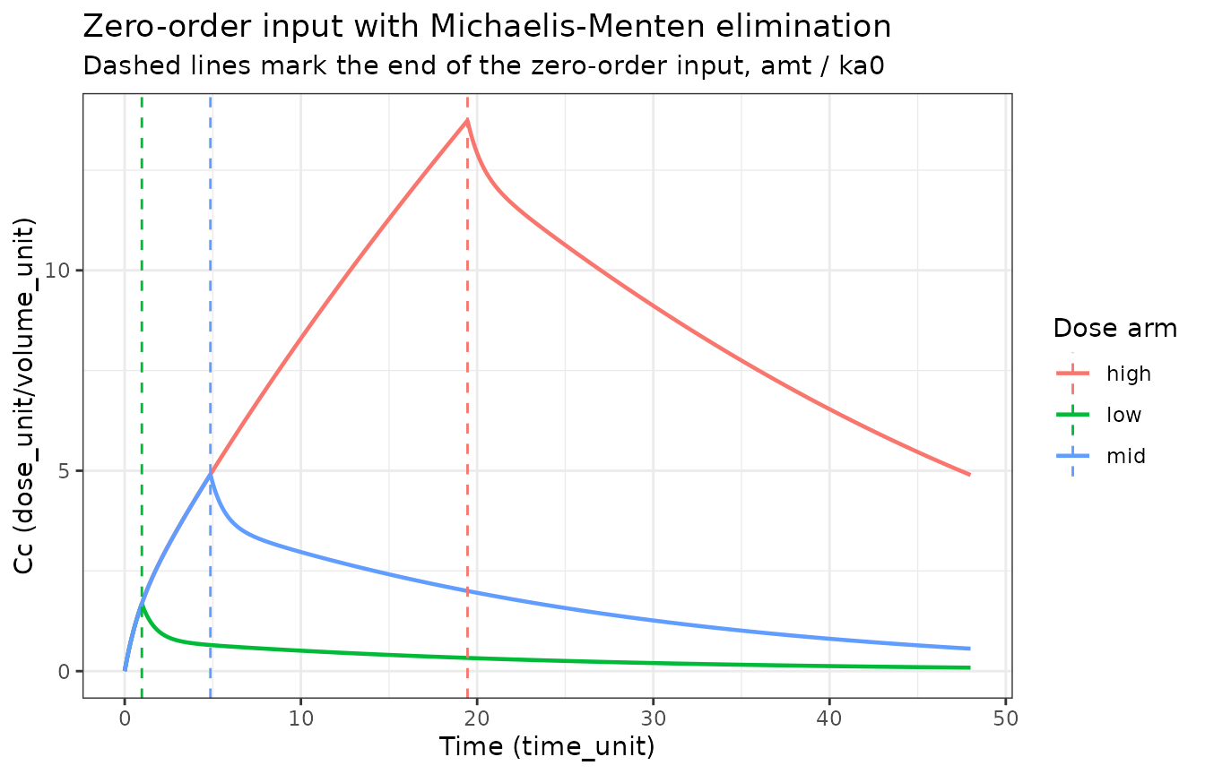

Structural validation

The paper reports no NCA table, no VPC of this toy model and no figure with digitisable values, so there is nothing to replicate numerically. What can be checked is that the encoded structure is the structure the supplement describes. Four closed-form gates do that, and each is paired with a control that proves the gate is not vacuous.

Gate 1 – the ODEs are solved, not silently replaced

rxode2 replaces an explicit d/dt system with an analytic linear solution when it recognises a cl / vc pair. This model deliberately has no cl, so the Michaelis-Menten arm cannot be discarded. Assert it.

stopifnot(is.null(mod$linCmt))
stopifnot(identical(mod$state, c("central", "peripheral1")))

Gate 2 – exact mass balance, including the zero-order input rate

Appending an accumulator state for eliminated amount closes the system: at any time, central + peripheral1 + eliminated must equal the amount delivered so far, which for a zero-order input of rate ka0 is min(t * ka0, amt). This gate validates the elimination expression and the reading of ka0 as a rate in a single identity, and it holds to solver tolerance rather than to a hand-chosen percentage.

mod_mb <- rxode2::model(
  mod,
  d / dt(eliminated) <- vmax * Cc / (km + Cc),
  append = TRUE
)

sim_mb <- rxode2::rxSolve(mod_mb, events, returnType = "data.frame")
#> Warning: multi-subject simulation without without 'omega'
sim_mb$dose <- as.numeric(doses)[sim_mb$id]

mb_err <- with(
  sim_mb,
  abs((central + peripheral1 + eliminated) - pmin(time * r1, dose))
)
max_mb_err <- max(mb_err)
max_mb_err
#> [1] 1.392664e-12

stopifnot(max_mb_err < 1e-8)

Control: the same identity computed against a deliberately-wrong input rate must fail by a wide margin. If it did not, the gate would be measuring nothing.

mb_err_mutated <- with(
  sim_mb,
  abs((central + peripheral1 + eliminated) - pmin(time * r1 * 0.9, dose))
)
max(mb_err_mutated)
#> [1] 19.9946

stopifnot(max(mb_err_mutated) > 1)

Gate 3 – Tmax falls at the end of the zero-order input

While a zero-order input is running, the central compartment gains mass at the constant rate ka0; these parameter values keep that rate above the combined distribution and elimination losses throughout, so the peak sits exactly at the end of infusion. This is the signature that distinguishes a zero-order input from the bolus that a missing rate = -1 flag would silently produce.

tmax_obs <- vapply(
  seq_along(doses),
  function(i) {
    si <- sim[sim$id == i, ]
    si$time[which.max(si$Cc)]
  },
  numeric(1)
)

data.frame(
  treatment = names(doses),
  tmax_observed = tmax_obs,
  t_inf_expected = as.numeric(t_inf)
)
#>   treatment tmax_observed t_inf_expected
#> 1       low          0.95      0.9727626
#> 2       mid          4.85      4.8638132
#> 3      high         19.45     19.4552529

# Agreement to within one step of the 0.05 observation grid.
stopifnot(all(abs(tmax_obs - as.numeric(t_inf)) <= 0.05))

Control: dosing the same amounts as a bolus (no rate flag, so rate(central) is never consulted) must put every Tmax at time 0.

events_bolus <- events
events_bolus$rate[events_bolus$evid == 1] <- 0
sim_bolus <- rxode2::rxSolve(mod, events_bolus, returnType = "data.frame")
#> Warning: multi-subject simulation without without 'omega'

tmax_bolus <- vapply(
  seq_along(doses),
  function(i) {
    si <- sim_bolus[sim_bolus$id == i, ]
    si$time[which.max(si$Cc)]
  },
  numeric(1)
)
tmax_bolus
#> [1] 0 0 0

stopifnot(all(tmax_bolus == 0))

Gate 4 – elimination saturates

With Michaelis-Menten elimination and no linear clearance term, exposure must rise faster than proportionally with dose: dose-normalised AUC is strictly increasing. A linear model would hold it constant, so this gate discriminates the encoded elimination from the linear alternative.

auc_trap <- function(time, conc) {
  sum(diff(time) * (head(conc, -1) + tail(conc, -1)) / 2)
}

dn_auc <- vapply(
  seq_along(doses),
  function(i) {
    si <- sim[sim$id == i, ]
    auc_trap(si$time, si$Cc) / doses[[i]]
  },
  numeric(1)
)

data.frame(treatment = names(doses), dose = as.numeric(doses), dn_auc = dn_auc)
#>   treatment dose   dn_auc
#> 1       low   10 1.642044
#> 2       mid   50 1.759391
#> 3      high  200 1.953727

stopifnot(all(diff(dn_auc) > 0))

# The peak concentration of the top arm must reach the saturable regime,
# otherwise the Michaelis-Menten arm is never exercised at all.
stopifnot(max(sim$Cc[sim$id == 3]) > km / 2)

PKNCA validation

PKNCA provides the independent NCA arm. It is run here as a cross-check of the simulated profiles rather than as a comparison against published values, because the source reports no NCA (see Errata).

sim_nca <-
  sim |>
  dplyr::filter(!is.na(Cc)) |>
  dplyr::select(id, time, Cc, treatment)

# Time-zero anchor: pre-dose concentration is 0 for a zero-order input.
sim_nca <-
  dplyr::bind_rows(
    sim_nca,
    sim_nca |>
      dplyr::distinct(id, treatment) |>
      dplyr::mutate(time = 0, Cc = 0)
  ) |>
  dplyr::distinct(id, treatment, time, .keep_all = TRUE) |>
  dplyr::arrange(id, time)

dose_df <-
  events |>
  dplyr::filter(evid == 1) |>
  dplyr::mutate(time = 0) |>
  dplyr::select(id, time, amt, treatment)

conc_obj <- PKNCA::PKNCAconc(
  sim_nca, Cc ~ time | treatment + id,
  concu = "dose_unit/volume_unit", timeu = "time_unit"
)
dose_obj <- PKNCA::PKNCAdose(
  dose_df, amt ~ time | treatment + id,
  doseu = "dose_unit"
)

intervals <- data.frame(
  start = 0, end = 48,
  cmax = TRUE, tmax = TRUE, auclast = TRUE, clast.obs = TRUE
)

res <- PKNCA::pk.nca(PKNCA::PKNCAdata(conc_obj, dose_obj, intervals = intervals))
nca_wide <-
  as.data.frame(res) |>
  dplyr::select(treatment, PPTESTCD, PPORRES) |>
  tidyr::pivot_wider(names_from = PPTESTCD, values_from = PPORRES)

nca_wide |>
  dplyr::rename(
    "Dose arm" = treatment,
    "Cmax (dose_unit/volume_unit)" = cmax,
    "Tmax (time_unit)" = tmax,
    "AUC0-48 (dose_unit*time_unit/volume_unit)" = auclast,
    "Clast (dose_unit/volume_unit)" = clast.obs
  ) |>
  knitr::kable(digits = 3)

Dose arm	AUC0-48 (dose_unit*time_unit/volume_unit)	Cmax (dose_unit/volume_unit)	Tmax (time_unit)	Clast (dose_unit/volume_unit)
high	390.745	13.737	19.45	4.894
low	16.420	1.657	0.95	0.087
mid	87.969	4.899	4.85	0.561

PKNCA must agree with the structural gates computed above: its tmax is the end of the zero-order input, and its dose-normalised auclast is strictly increasing across the ladder.

nca_ord <- nca_wide[match(names(doses), nca_wide$treatment), ]

stopifnot(all(abs(nca_ord$tmax - as.numeric(t_inf)) <= 0.05))
stopifnot(all(diff(nca_ord$auclast / as.numeric(doses)) > 0))

Comparison against published NCA

None is possible. Ibrahim 2019 reports dOFVBias, the CWRES bias vector b, %delta and % known bias for its diagnostic; it reports no Cmax, Tmax, AUC or half-life for the simple PK example, and no concentration figure with digitisable axes. The structural gates above stand in place of a published-NCA comparison.

Assumptions and deviations

Errata and gaps in the source.

No units anywhere. Table 1 of the supplement gives six bare numbers. The model’s units metadata therefore uses the placeholder tokens time_unit / dose_unit / volume_unit so that an assumed unit can never be mistaken for a published one.
No dose and no sampling schedule. The dose ladder (10 / 50 / 200) and the 0-48 observation grid in this vignette are demonstration choices made here, selected so the peak of the top arm exceeds KM / 2 and the Michaelis-Menten arm is genuinely exercised. They are not the authors’ design, which is unreported.
No inter-individual variability. The supplement states that 100 subjects were simulated, which implies random effects, but reports no omega for any parameter. Per policy, variances are never invented: the model is typical-value-only and carries no eta terms. A user who wants a cohort must supply their own omegas.
No residual error. No sigma is reported either; addSd is fixed(0).
ka0 is read as an input RATE, not a duration. This is the one interpretive call in the extraction. The supplement’s own footnote reads “ka0 zero order absorption rate”, and the library’s canonical encoding for a zero-order input rate is lr1 / r1 applied through rate(<cmt>) (as in Brekkan_2018_pegfilgrastim, Lin_2023_asparaginaseErwiniaRecombinant, Sager_2023_sotrovimab and Wang_2022_aripiprazole). The alternative reading – ka0 as a zero-order duration, the canonical ld1 / d1 applied through dur(<cmt>) – cannot be excluded from the source text alone, because no dose is given against which a duration could be checked. The printed row label is the only evidence, and it says “rate”.
The misspecified companion model is not packaged. The supplement describes it exactly (“the same as the simulation model except for using 1st order absorption process instead of the true zero order absorption process”) and reports its dOFVBias of -165.8, but publishes no parameter estimates for it. Its ini() would be empty, so it is not a model in the sense this library packages.

The deposited files in Supplementary Material 2 (miss.ext, miss_linbase.dta, extra_table, Bias_calculations.r) do not close that gap, and were checked rather than assumed. They belong to a different worked example of the R implementation: the data set carries 26 subjects, not 100, its population predictions are reproduced essentially exactly by a first-order-absorption structure with Vc near 2.2 and KM near 49 (sum of squares 1.3e-3 over 136 points) and not at all by the constants in Table 1, and no permutation of the six THETA values in miss.ext reproduces those predictions (best-permutation sum of squares 1.7e2). miss.ext is the linearised model’s parameter file, so its THETA indices are not the PK parameters and cannot be mapped onto them.
The IGI and IMM models of the main text are not packaged. Ibrahim 2019 uses them as demonstration vehicles and reports only dOFVBias (Table I) and CWRES bias estimates (Table II) for them – no structural parameter values at all. They are separate primary sources: Silber 2007 (https://doi.org/10.1177/0091270007304457) for the IGI model and Largajolli 2013 (PAGE 22, Abstract 2762) for the integrated minimal model.

No deviations from library convention. All parameter names (lvc, lvp, lq, lvmax, lkm, lr1, addSd) and compartment names (central, peripheral1) are canonical; checkModelConventions() is clean.