Growth curves in youth-onset type 2 diabetes (Hosey 2022)
Source:vignettes/articles/Hosey_2022_t2dm_growth.Rmd
Hosey_2022_t2dm_growth.RmdModel and source
- Citation: Hosey CM, Halpin K, Shakhnovich V, Bi C, Sweeney B, Yan Y, Leeder JS. Pediatric growth patterns in youth-onset type 2 diabetes mellitus: Implications for physiologically-based pharmacokinetic models. Clin Transl Sci. 2022;15(4):912-922. doi:10.1111/cts.13207.
- Article (open access, PMC9010268): https://doi.org/10.1111/cts.13207
Hosey 2022 is not a drug model. It supplies the anthropometric system layer for pediatric physiologically based pharmacokinetic (PBPK) models of youth with type 2 diabetes mellitus (T2DM). PBPK scaling factors such as liver volume are functions of body surface area, and so of height and weight. The standard CDC growth charts describe typically developing children and stop at the 97th percentile, which leaves most children with T2DM outside them. The authors therefore refitted the CDC functional forms to the heights and weights of children who developed T2DM:
- Height uses the CDC three-logistic stature function
- Weight uses the CDC polynomial , where the term is present for males only.
Both equations are fitted separately for each sex, with age in years.
In the model, the rxode2 time variable is
chronological age in years. The model has two outputs, ht
(cm) and bw (kg). Each carries a proportional residual
error equal to the sex- and output-specific coefficient of variation of
the held-out validation set (Table 2). These are the SD bands that
Figure 2 draws around each curve.
Population
- species: human
- n_subjects: 356
- n_studies: 1
- age_range: 2 to 18 years (target population); data from 19 to 25 years were also used in model development to stabilise the curves at older ages (Methods, Dataset)
- sex_female_pct: 59.3
- race_ethnicity: Self-identified: female 41.7% White, 32.2% Black, 15.7% Hispanic, 2.8% Asian, 5.2% multiple, 1.9% other/unknown; male 53.1% White, 20.7% Black, 14.5% Hispanic, 4.1% Asian, 3.5% multiple, 4.1% other/unknown (Supplemental Information S4)
- disease_state: Youth with a diagnosis of type 2 diabetes mellitus (ICD-9 / ICD-10 codes), most with overweight or obesity; children with type 1 diabetes were excluded. Visits both before and after the type 2 diabetes diagnosis were included (Methods, Dataset).
- dose_range: n/a (no drug)
- regions: United States (Children’s Mercy Kansas City, Kansas and Missouri)
- n_female: 211
- n_male: 145
- n_height_points: female 3973 training + 458 validation; male 2610 training + 306 validation (Table 1)
- n_weight_points: female 5189 training + 576 validation; male 3350 training + 380 validation (Table 1)
- notes: Deidentified electronic-medical-record height, weight, age and sex from visits recorded 2010-01-01 to 2016-08-24 (with some older records converted back to 1997). Data were binned in 6-month intervals and pruned with the modified Thompson-Tau algorithm; 90% of the data were used for development (100 x 5-fold cross validation with an iteratively reweighted least squares robust M-estimator, robustbase::nlrob) and 10% were held out for validation. Weight coefficients are the average over the 500 cross-validation fits; the height curve was refitted through the averaged monthly predictions (Methods, Model development).
The data are 356 children (211 female, 145 male) with an ICD-9 / ICD-10 diagnosis of T2DM seen at Children’s Mercy Kansas City (Table 1). Children with type 1 diabetes were excluded. Visits before and after the T2DM diagnosis were both used, so the curves describe the growth of children who develop T2DM, not only growth after diagnosis. The target range is 2 to 18 years. Data from 19 to 25 years were added only to keep the curves from dropping off at the upper end (Methods, Dataset). Supplemental Information S4 gives the self-identified race and ethnicity distribution.
Source trace
Each ini() entry in
inst/modeldb/endogenous/Hosey_2022_t2dm_growth.R has an
in-file comment giving its origin. The table below collects them in one
place.
| Model component | Source location |
|---|---|
Height equation form (ht_male,
ht_female) |
Methods, “Model development” (CDC stature function) |
ht_a_male … ht_c3_male (166, 0.283, 0.717,
5.18, 1.44, 0.245, 5.11, 178, 1.8, 12.4) |
Results, “Male height (cm, age in years)” equation |
ht_a_female … ht_c3_female (160, 0.396,
0.604, 0.537, 2.23, 0.0039, 1.77, 209, 0.473, 9.54) |
Results, “Female height (cm, age in years)” equation |
Weight equation form (bw_male,
bw_female) |
Methods, “Model development” (CDC weight polynomial) |
bw_a_male … bw_k_male
|
Supplemental Information S1, column “Male” (six significant figures) |
bw_b_female … bw_k_female
|
Supplemental Information S1, column “Female” (six significant figures; no term) |
propSd_ht_male 0.0587, propSd_ht_female
0.0675 |
Table 2, “Coefficients of variation (%)”, Height, column “Validation set fit to growth model: T2DM” |
propSd_bw_male 0.378, propSd_bw_female
0.459 |
Table 2, “Coefficients of variation (%)”, Weight, same column |
| Proportional form of the residual error | Figure 2 caption (SD bands “derived from the coefficient of variation (%) of the datapoints from the model”); checked numerically below |
Sex selection via SEXF
|
Separate male / female equations throughout Results and S1 |
Units
| Symbol | Units | Note |
|---|---|---|
time / age
|
year | the rxode2 time variable is chronological age |
ht, ht_male, ht_female
|
cm | standing height (stature) |
bw, bw_male, bw_female
|
kg | |
ht_a_*, ht_f_*
|
cm | |
ht_q_*, ht_p_*
|
fraction | for both sexes as printed |
ht_b1_*, ht_b2_*,
ht_b3_*
|
1/year | |
ht_c1_*, ht_c2_*,
ht_c3_*
|
year | |
bw_<x>_* for the coefficient of
|
kg/year^n | |
propSd_* |
fraction |
Parameter table
| Parameter | Value | Fixed in source | Label |
|---|---|---|---|
| ht_a_male | 166.0000000 | TRUE | Height curve coefficient a, male (cm) |
| ht_q_male | 0.2830000 | TRUE | Height curve fraction q of a in the first logistic, male (fraction) |
| ht_p_male | 0.7170000 | TRUE | Height curve fraction p of a in the second logistic, male (fraction) |
| ht_b1_male | 5.1800000 | TRUE | Height curve first-logistic rate b1, male (1/year) |
| ht_c1_male | 1.4400000 | TRUE | Height curve first-logistic midpoint c1, male (year) |
| ht_b2_male | 0.2450000 | TRUE | Height curve second-logistic rate b2, male (1/year) |
| ht_c2_male | 5.1100000 | TRUE | Height curve second-logistic midpoint c2, male (year) |
| ht_f_male | 178.0000000 | TRUE | Height curve coefficient f, male (cm) |
| ht_b3_male | 1.8000000 | TRUE | Height curve third-logistic (pubertal) rate b3, male (1/year) |
| ht_c3_male | 12.4000000 | TRUE | Height curve third-logistic (pubertal) midpoint c3, male (year) |
| ht_a_female | 160.0000000 | TRUE | Height curve coefficient a, female (cm) |
| ht_q_female | 0.3960000 | TRUE | Height curve fraction q of a in the first logistic, female (fraction) |
| ht_p_female | 0.6040000 | TRUE | Height curve fraction p of a in the second logistic, female (fraction) |
| ht_b1_female | 0.5370000 | TRUE | Height curve first-logistic rate b1, female (1/year) |
| ht_c1_female | 2.2300000 | TRUE | Height curve first-logistic midpoint c1, female (year) |
| ht_b2_female | 0.0039000 | TRUE | Height curve second-logistic rate b2, female (1/year) |
| ht_c2_female | 1.7700000 | TRUE | Height curve second-logistic midpoint c2, female (year) |
| ht_f_female | 209.0000000 | TRUE | Height curve coefficient f, female (cm) |
| ht_b3_female | 0.4730000 | TRUE | Height curve third-logistic (pubertal) rate b3, female (1/year) |
| ht_c3_female | 9.5400000 | TRUE | Height curve third-logistic (pubertal) midpoint c3, female (year) |
| bw_a_male | 0.0000000 | TRUE | Weight polynomial coefficient a (age^10), male (kg/year^10) |
| bw_b_male | -0.0000046 | TRUE | Weight polynomial coefficient b (age^9), male (kg/year^9) |
| bw_c_male | 0.0002609 | TRUE | Weight polynomial coefficient c (age^8), male (kg/year^8) |
| bw_d_male | -0.0083563 | TRUE | Weight polynomial coefficient d (age^7), male (kg/year^7) |
| bw_e_male | 0.1658670 | TRUE | Weight polynomial coefficient e (age^6), male (kg/year^6) |
| bw_f_male | -2.1208800 | TRUE | Weight polynomial coefficient f (age^5), male (kg/year^5) |
| bw_g_male | 17.5837000 | TRUE | Weight polynomial coefficient g (age^4), male (kg/year^4) |
| bw_h_male | -92.5981000 | TRUE | Weight polynomial coefficient h (age^3), male (kg/year^3) |
| bw_i_male | 293.8230000 | TRUE | Weight polynomial coefficient i (age^2), male (kg/year^2) |
| bw_j_male | -499.9800000 | TRUE | Weight polynomial coefficient j (age), male (kg/year) |
| bw_k_male | 358.4400000 | TRUE | Weight polynomial intercept k, male (kg) |
| bw_b_female | -0.0000005 | TRUE | Weight polynomial coefficient b (age^9), female (kg/year^9) |
| bw_c_female | 0.0000500 | TRUE | Weight polynomial coefficient c (age^8), female (kg/year^8) |
| bw_d_female | -0.0021933 | TRUE | Weight polynomial coefficient d (age^7), female (kg/year^7) |
| bw_e_female | 0.0529444 | TRUE | Weight polynomial coefficient e (age^6), female (kg/year^6) |
| bw_f_female | -0.7703050 | TRUE | Weight polynomial coefficient f (age^5), female (kg/year^5) |
| bw_g_female | 6.9562500 | TRUE | Weight polynomial coefficient g (age^4), female (kg/year^4) |
| bw_h_female | -38.7195000 | TRUE | Weight polynomial coefficient h (age^3), female (kg/year^3) |
| bw_i_female | 127.5240000 | TRUE | Weight polynomial coefficient i (age^2), female (kg/year^2) |
| bw_j_female | -221.1400000 | TRUE | Weight polynomial coefficient j (age), female (kg/year) |
| bw_k_female | 164.3030000 | TRUE | Weight polynomial intercept k, female (kg) |
| propSd_ht_male | 0.0587000 | TRUE | Proportional residual SD of height, male (fraction) |
| propSd_ht_female | 0.0675000 | TRUE | Proportional residual SD of height, female (fraction) |
| propSd_bw_male | 0.3780000 | TRUE | Proportional residual SD of body weight, male (fraction) |
| propSd_bw_female | 0.4590000 | TRUE | Proportional residual SD of body weight, female (fraction) |
All coefficients are the paper’s final point estimates from robust
nonlinear regression, reported without uncertainty. The CVs are summary
statistics of the validation set. Every value is therefore
fixed().
Simulation
Typical curves
The typical-value outputs ht and bw do not
depend on the residual error, so they are read directly from the solved
columns. One “subject” per sex is solved on a fine age grid.
mod <- readModelDb("Hosey_2022_t2dm_growth")

solve_sex <- function(sexf, ages) {
  ev <- data.frame(id = 1L, time = ages, evid = 0L, dvid = 1L, SEXF = sexf)
  out <- rxode2::rxSolve(mod, ev, returnType = "data.frame")
  out$SEXF <- sexf
  out$sex <- ifelse(sexf == 1, "Female", "Male")
  out
}

ages_fine <- seq(2, 25, by = 0.01)
typ <- dplyr::bind_rows(solve_sex(1, ages_fine), solve_sex(0, ages_fine))
nrow(typ)
#> [1] 4602
Stochastic cohort
A cross-sectional virtual cohort has 200 children per sex at each of
seven ages. Each row draws a height (dvid = 1) and a weight
(dvid = 2) with the proportional residual error. This is
how the paper’s Supplemental Information S3 Simcyp simulation used the
equations and the CVs.
rxode2::rxSetSeed(20220101)
ages_vpc <- c(2, 5, 8, 11, 14, 16, 18)
n_per_sex <- 200
cohort <- expand.grid(
  id = seq_len(2 * n_per_sex),
  time = ages_vpc,
  dvid = 1:2
) |>
  dplyr::mutate(
    evid = 0L,
    SEXF = as.integer(.data$id > n_per_sex)
  ) |>
  dplyr::arrange(.data$id, .data$time, .data$dvid)

vpc <- rxode2::rxSolve(mod, cohort, keep = "SEXF", returnType = "data.frame") |>
  dplyr::mutate(
    output = ifelse(.data$CMT == 1, "Height (cm)", "Weight (kg)"),
    pred = ifelse(.data$CMT == 1, .data$ht, .data$bw),
    sex = ifelse(.data$SEXF == 1, "Female", "Male")
  )
#> Warning: multi-subject simulation without without 'omega'
nrow(vpc)
#> [1] 5600
Validation
1. The model returns the published equations
The outputs must equal the printed equations, evaluated by hand here from the paper’s numbers, to machine precision. Both sides use the same coefficients, so any difference is transcription or algebra error and the bound is tight.
ht_eq <- function(age, a, q, p, b1, c1, b2, c2, f, b3, c3) {
  a * q / (1 + exp(-b1 * (age - c1))) +
    a * p / (1 + exp(-b2 * (age - c2))) +
    (f - a) / (1 + exp(-b3 * (age - c3)))
}
wt_male_s1 <- c(3.44781e-08, -4.57950e-06, 2.60885e-04, -8.35633e-03, 1.65867e-01,
                -2.12088, 17.5837, -92.5981, 293.823, -499.980, 358.440)
wt_female_s1 <- c(0, -4.81428e-07, 5.00192e-05, -2.19327e-03, 5.29444e-02,
                  -0.770305, 6.95625, -38.7195, 127.524, -221.140, 164.303)
wt_eq <- function(age, coefs) vapply(age, function(x) sum(coefs * x^(10:0)), numeric(1))

chk_ages <- c(2, 4, 6, 8, 10, 12, 14, 16, 18)
chk <- typ |>
  dplyr::filter(round(.data$time, 2) %in% chk_ages) |>
  dplyr::mutate(
    ht_hand = ifelse(
      .data$SEXF == 1,
      ht_eq(.data$time, 160, 0.396, 0.604, 0.537, 2.23, 0.0039, 1.77, 209, 0.473, 9.54),
      ht_eq(.data$time, 166, 0.283, 0.717, 5.18, 1.44, 0.245, 5.11, 178, 1.8, 12.4)
    ),
    bw_hand = ifelse(
      .data$SEXF == 1,
      wt_eq(.data$time, wt_female_s1),
      wt_eq(.data$time, wt_male_s1)
    )
  )
stopifnot(
  nrow(chk) == 2 * length(chk_ages),
  all(abs(chk$ht - chk$ht_hand) < 1e-8),
  all(abs(chk$bw - chk$bw_hand) < 1e-8)
)
chk |>
  dplyr::select("sex", "time", "ht", "bw") |>
  dplyr::rename("Sex" = "sex", "Age (y)" = "time", "Height (cm)" = "ht", "Weight (kg)" = "bw") |>
knitr::kable(digits = 1)| Sex | Age (y) | Height (cm) | Weight (kg) |
|---|---|---|---|
| Female | 2 | 79.4 | 12.1 |
| Female | 4 | 97.6 | 18.2 |
| Female | 6 | 112.4 | 25.7 |
| Female | 8 | 125.5 | 37.8 |
| Female | 10 | 138.6 | 50.0 |
| Female | 12 | 149.6 | 60.6 |
| Female | 14 | 156.4 | 77.0 |
| Female | 16 | 159.8 | 94.1 |
| Female | 18 | 161.3 | 91.9 |
| Male | 2 | 82.4 | 16.1 |
| Male | 4 | 98.4 | 21.5 |
| Male | 6 | 113.0 | 25.1 |
| Male | 8 | 126.7 | 34.7 |
| Male | 10 | 138.6 | 49.3 |
| Male | 12 | 151.4 | 67.6 |
| Male | 14 | 165.3 | 92.5 |
| Male | 16 | 170.3 | 109.1 |
| Male | 18 | 173.1 | 96.8 |
2. Height velocity, replicating Figure 5
The Methods define height velocity as the first derivative of the final height models. Results reports a local peak of height velocity at 8.5 years for females and 12.5 years for males. The paper binned its results in 6-month intervals, so the peak is compared at that resolution.
vel <- typ |>
  dplyr::group_by(.data$sex) |>
  dplyr::arrange(.data$time, .by_group = TRUE) |>
  dplyr::mutate(velocity = (dplyr::lead(.data$ht) - dplyr::lag(.data$ht)) /
    (dplyr::lead(.data$time) - dplyr::lag(.data$time))) |>
  dplyr::ungroup() |>
  dplyr::filter(!is.na(.data$velocity))

# A LOCAL maximum: velocity above both neighbours. The female curve is
# still falling from its early-childhood value at 6 years, so a plain
# window maximum would return the window edge instead of the peak.
local_max <- vel |>
  dplyr::group_by(.data$sex) |>
  dplyr::filter(
    .data$velocity > dplyr::lag(.data$velocity),
    .data$velocity > dplyr::lead(.data$velocity),
    .data$time > 3
  ) |>
  dplyr::ungroup()
# Males also have a shallow mid-childhood maximum near 5 years; the
# pubertal peak is the larger one.
stopifnot(all(c("Female", "Male") %in% local_max$sex))
peaks <- local_max |>
  dplyr::group_by(.data$sex) |>
  dplyr::slice_max(.data$velocity, n = 1) |>
  dplyr::ungroup() |>
  dplyr::arrange(.data$sex) |>
  dplyr::mutate(published = c(8.5, 12.5)) |>
  dplyr::select("sex", "time", "velocity", "published")
stopifnot(all(abs(peaks$time - peaks$published) <= 0.5))
peaks |>
  dplyr::rename(
    "Sex" = "sex", "Model peak age (y)" = "time",
    "Peak velocity (cm/y)" = "velocity", "Published peak age (y)" = "published"
  ) |>
knitr::kable(digits = 2)| Sex | Model peak age (y) | Peak velocity (cm/y) | Published peak age (y) |
|---|---|---|---|
| Female | 8.75 | 6.66 | 8.5 |
| Male | 12.33 | 9.01 | 12.5 |
vel |>
  dplyr::filter(.data$time >= 2.5, .data$time <= 24.5) |>
  ggplot(aes(.data$time, .data$velocity)) +
  geom_line() +
  facet_wrap(~sex) +
  labs(x = "Age (years)", y = "Height velocity (cm/year)") +
  coord_cartesian(ylim = c(0, 10)) +
  theme_bw()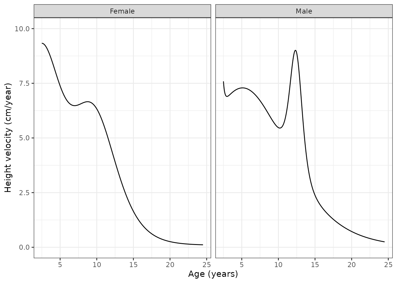
Replicates Figure 5 of Hosey 2022: height velocity of the T2DM-specific height curves, females (left) and males (right). The published solid lines start near 9.3 (female) and 7.6 (male) cm/year at 2.5 years, peak near 6.6 cm/year at 8.5 years (female) and 8.9 cm/year at 12.5 years (male), and decline towards zero by 25 years.
On the 0.01-year grid the model’s pubertal peaks fall at 8.75 years (female, 6.66 cm/year) and 12.33 years (male, 9.0 cm/year). Both are within the 6-month binning of the published 8.5 and 12.5 years. The start of the curves at 2.5 years (female 9.3, male 7.6 cm/year) also agrees with the Figure 5 panels. The small female (0.0039 per year) is consistent with Figure 5 as printed. It makes the second logistic almost linear, and it gives the slow residual female velocity of about 0.1 cm/year still visible at 24 years.
3. Curves against Figure 2
The maintainers digitised the red “patient-specific model” curves of Figure 2 at whole-year ages, from the article PDF rendered at 250 dpi with axes calibrated on the tick marks. These values are read off a figure, not published numbers. Reading error is about 0.5 cm for height and about 1 kg for weight.
fig2 <- tibble::tibble(
  time = rep(2:18, 4),
  sex = rep(c("Female", "Male", "Female", "Male"), each = 17),
  output = rep(c("ht", "ht", "bw", "bw"), each = 17),
  digitised = c(
    # Figure 2a, height, females
    80.6, 89.1, 97.9, 106.1, 113.5, 119.9, 126.1, 133.6, 140.4, 145.2, 149.3,
    153.9, 156.6, 158.4, 159.7, 160.7, 161.5,
    # Figure 2b, height, males
    83.5, 92.1, 98.7, 105.7, 113.4, 120.8, 127.2, 133.0, 138.6, 145.1, 151.9,
    158.9, 164.7, 168.5, 170.9, 172.6, 173.5,
    # Figure 2c, weight, females
    11.5, 13.7, 18.0, 21.7, 26.0, 31.2, 38.2, 44.9, 51.6, 57.9, 64.0, 70.7,
    78.3, 87.6, 96.1, 102.2, 104.1,
    # Figure 2d, weight, males
    13.2, 16.7, 20.4, 23.6, 26.0, 29.1, 34.9, 43.0, 51.4, 60.3, 69.4, 79.2,
    89.6, 98.5, 106.3, 116.3, 124.7
  )
)

cmp <- typ |>
  dplyr::filter(round(.data$time, 2) %in% 2:18) |>
  dplyr::mutate(time = round(.data$time)) |>
  dplyr::select("time", "sex", "ht", "bw") |>
  tidyr::pivot_longer(c("ht", "bw"), names_to = "output", values_to = "model") |>
  dplyr::inner_join(fig2, by = c("time", "sex", "output")) |>
  dplyr::mutate(pct_diff = 100 * (.data$model - .data$digitised) / .data$digitised)
stopifnot(nrow(cmp) == nrow(fig2))

# Height: the printed three-significant-figure logistic coefficients
# reproduce the figure at every age.
cmp_ht <- dplyr::filter(cmp, .data$output == "ht")
stopifnot(all(abs(cmp_ht$pct_diff) < 3))

# Weight: the S1 polynomial reproduces the figure over the core of the age
# range (4 to 16 years). The edges diverge; see the Errata.
cmp_bw_core <- dplyr::filter(cmp, .data$output == "bw", .data$time >= 4, .data$time <= 16)
stopifnot(
  abs(median(cmp_bw_core$pct_diff)) < 3,
  all(abs(cmp_bw_core$pct_diff) < 10)
)

cmp |>
  dplyr::filter(.data$time %in% c(2, 3, 4, 6, 8, 10, 12, 14, 16, 17, 18)) |>
  dplyr::mutate(output = ifelse(.data$output == "ht", "Height (cm)", "Weight (kg)")) |>
  dplyr::arrange(.data$output, .data$sex, .data$time) |>
  dplyr::rename(
    "Output" = "output", "Sex" = "sex", "Age (y)" = "time",
    "Model" = "model", "Figure 2 (digitised)" = "digitised", "% difference" = "pct_diff"
  ) |>
knitr::kable(digits = 1)| Age (y) | Sex | Output | Model | Figure 2 (digitised) | % difference |
|---|---|---|---|---|---|
| 2 | Female | Height (cm) | 79.4 | 80.6 | -1.5 |
| 3 | Female | Height (cm) | 88.7 | 89.1 | -0.4 |
| 4 | Female | Height (cm) | 97.6 | 97.9 | -0.4 |
| 6 | Female | Height (cm) | 112.4 | 113.5 | -1.0 |
| 8 | Female | Height (cm) | 125.5 | 126.1 | -0.5 |
| 10 | Female | Height (cm) | 138.6 | 140.4 | -1.2 |
| 12 | Female | Height (cm) | 149.6 | 149.3 | 0.2 |
| 14 | Female | Height (cm) | 156.4 | 156.6 | -0.1 |
| 16 | Female | Height (cm) | 159.8 | 159.7 | 0.0 |
| 17 | Female | Height (cm) | 160.7 | 160.7 | 0.0 |
| 18 | Female | Height (cm) | 161.3 | 161.5 | -0.1 |
| 2 | Male | Height (cm) | 82.4 | 83.5 | -1.3 |
| 3 | Male | Height (cm) | 91.4 | 92.1 | -0.7 |
| 4 | Male | Height (cm) | 98.4 | 98.7 | -0.3 |
| 6 | Male | Height (cm) | 113.0 | 113.4 | -0.4 |
| 8 | Male | Height (cm) | 126.7 | 127.2 | -0.4 |
| 10 | Male | Height (cm) | 138.6 | 138.6 | 0.0 |
| 12 | Male | Height (cm) | 151.4 | 151.9 | -0.4 |
| 14 | Male | Height (cm) | 165.3 | 164.7 | 0.3 |
| 16 | Male | Height (cm) | 170.3 | 170.9 | -0.4 |
| 17 | Male | Height (cm) | 171.9 | 172.6 | -0.4 |
| 18 | Male | Height (cm) | 173.1 | 173.5 | -0.2 |
| 2 | Female | Weight (kg) | 12.1 | 11.5 | 5.5 |
| 3 | Female | Weight (kg) | 13.6 | 13.7 | -1.0 |
| 4 | Female | Weight (kg) | 18.2 | 18.0 | 0.9 |
| 6 | Female | Weight (kg) | 25.7 | 26.0 | -1.2 |
| 8 | Female | Weight (kg) | 37.8 | 38.2 | -1.1 |
| 10 | Female | Weight (kg) | 50.0 | 51.6 | -3.1 |
| 12 | Female | Weight (kg) | 60.6 | 64.0 | -5.3 |
| 14 | Female | Weight (kg) | 77.0 | 78.3 | -1.7 |
| 16 | Female | Weight (kg) | 94.1 | 96.1 | -2.0 |
| 17 | Female | Weight (kg) | 96.4 | 102.2 | -5.7 |
| 18 | Female | Weight (kg) | 91.9 | 104.1 | -11.7 |
| 2 | Male | Weight (kg) | 16.1 | 13.2 | 21.7 |
| 3 | Male | Weight (kg) | 15.9 | 16.7 | -4.6 |
| 4 | Male | Weight (kg) | 21.5 | 20.4 | 5.2 |
| 6 | Male | Weight (kg) | 25.1 | 26.0 | -3.5 |
| 8 | Male | Weight (kg) | 34.7 | 34.9 | -0.5 |
| 10 | Male | Weight (kg) | 49.3 | 51.4 | -4.0 |
| 12 | Male | Weight (kg) | 67.6 | 69.4 | -2.6 |
| 14 | Male | Weight (kg) | 92.5 | 89.6 | 3.3 |
| 16 | Male | Weight (kg) | 109.1 | 106.3 | 2.7 |
| 17 | Male | Weight (kg) | 106.8 | 116.3 | -8.2 |
| 18 | Male | Weight (kg) | 96.8 | 124.7 | -22.4 |
bands <- typ |>
  dplyr::filter(.data$time <= 18) |>
  dplyr::select("time", "sex", "ht", "bw", "propSd_ht", "propSd_bw") |>
  tidyr::pivot_longer(c("ht", "bw"), names_to = "output", values_to = "model") |>
  dplyr::mutate(
    cv = ifelse(.data$output == "ht", .data$propSd_ht, .data$propSd_bw),
    lo = .data$model * (1 - .data$cv),
    hi = .data$model * (1 + .data$cv)
  )
lab <- c(ht = "Height (cm)", bw = "Weight (kg)")
ggplot(bands, aes(.data$time)) +
  geom_line(aes(y = .data$model), colour = "firebrick") +
  geom_line(aes(y = .data$lo), colour = "firebrick", linetype = "dashed", alpha = 0.6) +
  geom_line(aes(y = .data$hi), colour = "firebrick", linetype = "dashed", alpha = 0.6) +
  geom_point(data = fig2, aes(y = .data$digitised), size = 1) +
  facet_grid(factor(output, levels = c("ht", "bw"), labels = lab) ~ sex, scales = "free_y") +
  labs(x = "Age (years)", y = NULL) +
  theme_bw()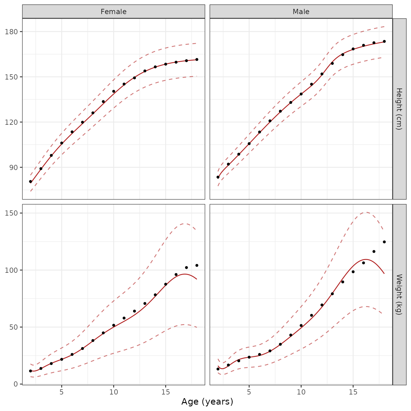
Replicates Figure 2 of Hosey 2022: T2DM-specific height and weight curves (solid) with the model x (1 +/- CV) bands (dashed), and the maintainers’ digitisation of the published red model curves (points). Panels are height and weight for females and males, as in Figure 2a-d.
The Figure 2 bands also confirm the residual-error form. The printed upper and lower pink lines at 18 years sit at about 173 and 151 cm (female height, curve 162 cm) and at about 172 and 78 kg (male weight, curve about 125 kg). Those are the curve multiplied by the Table 2 validation-set CVs (6.75% and 37.8%). This fixes both the proportional form and the Table 2 column the authors used.
4. Residual variability of the stochastic cohort
The spread of sim / pred in the virtual cohort must
recover the encoded CVs. Both sides come from the same draw, so the only
difference is Monte-Carlo error. With 1,400 draws per sex and output,
the standard error of an SD is about 2% of its value, and a 10%
tolerance leaves ample room.
cv_chk <- vpc |>
  dplyr::group_by(.data$output, .data$sex) |>
  dplyr::summarise(
    n = dplyr::n(),
    cv_sim = stats::sd(.data$sim / .data$pred),
    .groups = "drop"
  ) |>
  dplyr::mutate(cv_table2 = c(0.0675, 0.0587, 0.459, 0.378))
stopifnot(
  all(cv_chk$n == n_per_sex * length(ages_vpc)),
  all(abs(cv_chk$cv_sim / cv_chk$cv_table2 - 1) < 0.10)
)
cv_chk |>
  dplyr::rename(
    "Output" = "output", "Sex" = "sex", "N draws" = "n",
    "Simulated CV" = "cv_sim", "Table 2 CV" = "cv_table2"
  ) |>
knitr::kable(digits = 3)| Output | Sex | N draws | Simulated CV | Table 2 CV |
|---|---|---|---|---|
| Height (cm) | Female | 1400 | 0.069 | 0.068 |
| Height (cm) | Male | 1400 | 0.058 | 0.059 |
| Weight (kg) | Female | 1400 | 0.446 | 0.459 |
| Weight (kg) | Male | 1400 | 0.379 | 0.378 |
ggplot(vpc, aes(.data$time, .data$sim)) +
  geom_jitter(width = 0.2, alpha = 0.15, size = 0.6) +
  geom_line(
    data = bands |>
      dplyr::mutate(output = ifelse(.data$output == "ht", "Height (cm)", "Weight (kg)")),
    aes(.data$time, .data$model), colour = "firebrick"
  ) +
  facet_grid(output ~ sex, scales = "free_y") +
  labs(x = "Age (years)", y = NULL) +
  theme_bw()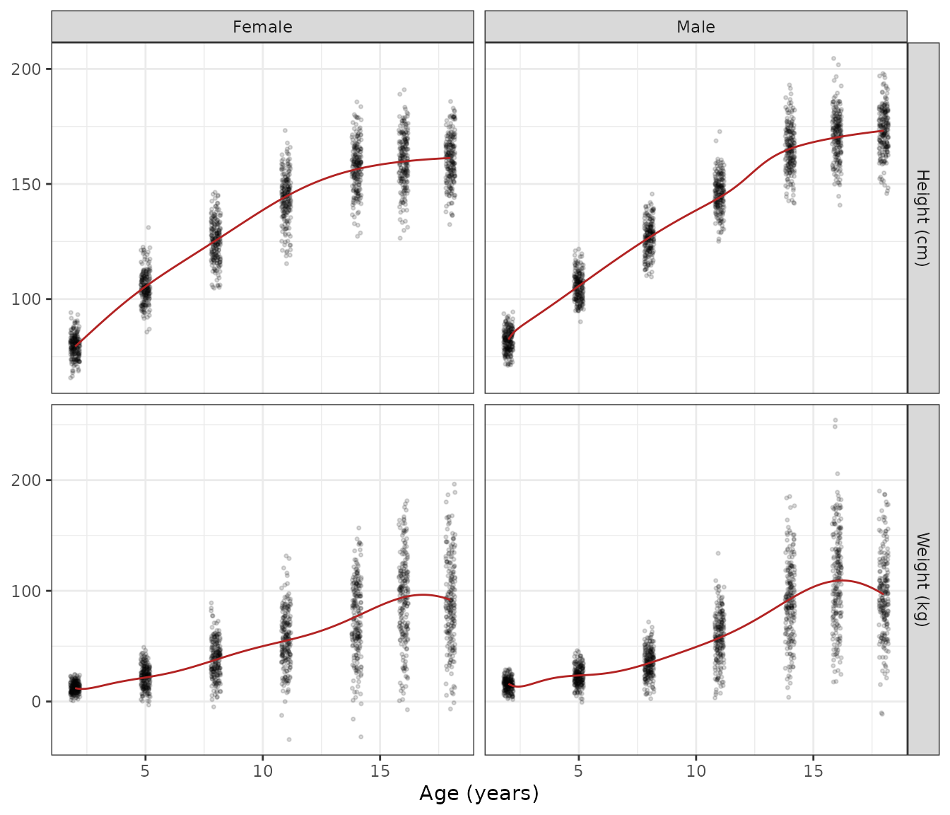
Virtual cross-sectional cohort (200 per sex at each age) simulated with the proportional residual error. This is analogous to the Simcyp simulation of Supplemental Information S3. Lines are the typical curves.
Because the error is proportional and normal, a weight CV near 40-46% gives a small fraction of non-physiological (near-zero or negative) weights in the lower tail. The paper’s Simcyp simulation carried the same CVs; users who need strictly positive draws should truncate or resample them.
Assumptions and deviations
-
Age is the time axis. The rxode2
timevariable is age in years. The model has no dosing and no ODE states. To use it as a covariate generator for a PBPK or popPK model, solve it on the age grid of interest and passht/bwon asHT/WTcovariates. - Weight coefficients come from Supplemental Information S1. The main-text weight equations are “truncated” to three significant figures and are not usable: they give about 420 kg for a 10-year-old boy. The paper itself says at least six significant figures are needed, and S1 supplies them.
-
The printed weight polynomials drift from Figure 2 at the
edges of the age range. Section 3 shows agreement within a few
percent from 4 to 16 years. Outside that range the printed coefficients
do not reproduce the published curve:
- Males at 2 years: the polynomial gives 16.1 kg against about 13 kg in Figure 2d. It also dips slightly between 2 and 3 years.
- 17 to 18 years: the polynomial turns down (male 96.8 kg and female 91.9 kg at 18 years) while Figure 2 keeps rising (about 125 and 104 kg).
- Height coefficients are the three-significant-figure values of the Results equations. No higher-precision height coefficients were published. The logistic form is well conditioned, and these values reproduce Figure 2a-b to within about 1% and Figure 5 closely.
- Residual error is proportional, with the validation-set CVs. Table 2 gives CVs both for the validation set fitted to the final model and for the cross-validation folds (for example, female weight 45.9% versus 44.6 +/- 0.92%). The validation-set column is used because it reproduces the Figure 2 SD bands. The CV is a pooled statistic, RMSE divided by the mean observation (for example, 26.3 kg / 0.459 = 57 kg mean female weight). Encoding it as a constant proportional error is the authors’ own use (Figure 2, Supplemental Information S3), not a per-age variance model.
- Not extracted: the CDC 50th-percentile comparator curves (not reproduced in the paper), the z-score analyses (Figures 3 and 4, descriptive), and the preliminary race/ethnicity curves of Supplemental Information S5 (no coefficients published).
- Errata: a check of EuropePMC and Crossref on 2026-09-30 found no erratum or correction for this article.