PI3K-inhibitor GI toxicity QSP model (Gadkar 2022)
Source:vignettes/articles/Gadkar_2022_pi3kiColitis_qsp.Rmd
Gadkar_2022_pi3kiColitis_qsp.RmdModel and source
mod <- rxode2::rxode(readModelDb("Gadkar_2022_pi3kiColitis_qsp"))- Citation: Gadkar K, Friedrich C, Hurez V, Ruiz M-L, Dickmann L, Jolly MK, Schutt L, Jin J, Ware JA, Ramanujan S. Quantitative systems pharmacology model-based investigation of adverse gastrointestinal events associated with prolonged treatment with PI3-kinase inhibitors. CPT Pharmacometrics Syst Pharmacol. 2022;11(5):616-627. doi:10.1002/psp4.12749. Equations: Supplement S10 (PSP4-11-616-s002.docx). Parameter values, dosing and per-drug variants: the authors’ deposited SimBiology project GI_risk_model.sbproj and Parameters.xlsx (PSP4-11-616-s001.zip).
- Description: QSP. Mechanistic model of colonic mucosal inflammation and epithelial barrier damage under prolonged PI3K-inhibitor treatment, used to predict the onset of diarrhea and colitis. A two-compartment oral (or IV bolus) PK model drives unbound mucosal and blood concentrations; the drug inhibits each PI3K isoform (alpha, beta, gamma, delta) through its own IC50, and the isoform activities modulate epithelial-cell formation and apoptosis, APC, effector-T-cell, Treg and neutrophil recruitment, activation, differentiation and proliferation, and IL-10 / IL-12 production. 21 ODE states: 3 PK states, 14 mucosal cell and cytokine states, an acute-injury stimulus (Activating_Event), a cumulative risk state (RISK), a tissue-exposure AUC and circulating natural Tregs. Outputs are the epithelial quality, the GI risk score (diarrhea onset when it exceeds 0.6) and RISK (colitis onset when it exceeds 200). Default parameters are the authors’ baseline virtual patient (SimBiology variant ‘VP0 (baseline VP)’) with taselisib PK and potency; the six other inhibitors (idelalisib, duvelisib, umbralisib, alpelisib, pictilisib, copanlisib) differ only in the PK, protein-binding and IC50 parameters listed in population$notes. The published incidences come from a prevalence-weighted virtual population of 704 parameter sets, which is not carried here; the model is deterministic.
- Article: https://doi.org/10.1002/psp4.12749 (open access)
The paper describes the model in prose and its Table 1. The full
equation list is in Supplement S10 of the supporting information. Every
parameter value, dose object and per-drug parameter set comes from the
authors’ deposited SimBiology project
(GI_risk_model.sbproj, Parameters.xlsx and
VPOP.mat, supporting-information archive
PSP4-11-616-s001.zip). The maintainers read these files
directly, and the reaction rates and rules in the project are identical
to the text of Supplement S10.
Population
The model is a quantitative systems pharmacology (QSP) representation of a cross-section of colonic mucosa (epithelium, lamina propria and gut-associated lymphoid tissue) plus a blood compartment that supplies immune cells. It was calibrated to clinical diarrhea and colitis incidences for six PI3K inhibitors: taselisib, idelalisib, duvelisib, umbralisib, alpelisib and pictilisib (paper Table 2). It was also calibrated to individual diarrhea- and colitis-onset times from a proprietary taselisib trial. Copanlisib was held out for validation.
Between-patient variability is represented by a prevalence-weighted
virtual population (VPop) of 704 virtual patients that vary 88
mechanistic parameters. This package carries only the authors’ baseline
virtual patient (VP0 (baseline VP)). The full VPop is a set
of 704 weighted parameter vectors, not a parametric distribution, so it
cannot be expressed as inter-individual variability. See the
reproduction section below for how the packaged equations perform
against it.
str(mod$population)
#> List of 7
#>  $ species      : chr "human (virtual population)"
#>  $ n_subjects   : int 704
#>  $ n_studies    : int NA
#>  $ disease_state: chr "Patients with cancer (solid tumours or B-cell malignancies) receiving PI3K inhibitors. Calibrated to the publis"| __truncated__
#>  $ dose_range   : chr "Deposited regimens: taselisib 4 mg QD, idelalisib 150 mg BID, duvelisib 25 mg BID, umbralisib 800 mg QD, alpeli"| __truncated__
#>  $ regions      : chr NA
#>  $ notes        : chr "The 704 virtual patients are prevalence-weighted parameter sets varying 88 mechanistic parameters (authors' VPO"| __truncated__
Source trace
| Equation / parameter | Value | Source location |
|---|---|---|
| Drug PK (depot, central, peripheral1; F flux, lag, zero-order input) | taselisib defaults | Supplement S10 fluxes PI3Ki_*; Table S5; deposited
variant Taselisib (GDC-0032) and dose
PI3Kinh_QD_4mg_Tablet
|
Cc = 1000 * central / vc (ng/mL) |
– | S10 rule
Blood.PI3K_Inh_circ_total = PI3Kinh_circ*1e6/(PI3Kinh_Vc*1000)
|
Cu = fu * Cc, fu = 1 - 0.76
|
0.24 | S10 rule Blood.PI3K_Inh_circ_conc; Table S5 bound
fraction |
Cmucosa = kp_gut * Cu, kp_gut
|
0.5 | S10 rule Mucosa.PI3K_Inhibitor; deposited
PI3Kinh_partition
|
Isoform activity 1 - imax * C / (ic50 + C)
|
– | S10 rules PI3Ka_EC, PI3Kd_APC, …
(identical per isoform across cell types) |
lic50_pi3ka/b/g/d (unbound, ng/mL) |
0.13 / 4 / 0.45 / 0.055 | Deposited taselisib variant; Table S3 (nM) |
| Mucosal fluxes (recruitment, activation, differentiation, proliferation, cytokine production and clearance) | – | Supplement S10 ‘Fluxes’ |
Epithelial_Quality = min(1, EChealthy + 0.2 * ECact) |
– | S10 ‘Repeated Assignments’; Table 1 |
GI_Risk_Score |
weights 0.2 / 0.8 | S10 ‘Repeated Assignments’; Table 1 |
d/dt(RISK) = k_healing * (GI - RISK * (GI < threshold)) |
– | S10 fluxes insult, healing
|
| 21 ODEs | – | Supplement S10 ‘ODEs’ |
| 155 mechanistic parameters | see model file |
Parameters.xlsx tab ‘All parameters’ (= variant
VP0 (baseline VP)); rounded values in Table S1 |
Diarrhea criterion max(GI_Risk_Score) > 0.6
|
0.6 | Table 1; getAE.m threshold0
|
Colitis criterion max(RISK) > 200
|
200 |
getAE.m threshold2 (Table 1 prints 120;
see Assumptions) |
| Initial conditions | drug-free steady state | Converged run-in of the deposited procedure
(simulate_Vpop.m) |
Per-drug parameters
The seven inhibitors share every mechanistic parameter. They differ only in their PK, protein binding and isoform IC50s, which the deposited project stores as one SimBiology variant per drug. The IC50s are unbound concentrations in ng/mL, which is Table S3 in nM times the molecular weight divided by 1000.
drugs <- tibble::tribble(
  ~drug,        ~cl,   ~vc,    ~q,     ~vp,   ~ka,   ~tlag, ~fb,    ~ic50a,   ~ic50b, ~ic50g, ~ic50d, ~amt, ~ii, ~route,
  "Taselisib",   5,     200,    10,     50,    0.7,   0.2,   0.76,   0.13,     4,      0.45,   0.055,  4,    24,  "oral",
  "Idelalisib",  14.88, 22.65,  11.82,  72.97, 0.482, 0.247, 0.84,   340.64,   234.71, 36.97,  1.04,   150,  12,  "oral",
  "Duvelisib",   5,     200,    10,     50,    0.7,   0.2,   0.7625, 667.81,   35.43,  11.26,  1.04,   25,   12,  "oral",
  "Umbralisib",  8.7,   550,    10,     160,   0.8,   0.2,   0.7625, 101200,   506,    485,    10.12,  800,  24,  "oral",
  "Alpelisib",   11.5,  118,    0,      1,     0.784, 0.489, 0.9,    2.21,     510,    128,    110,    300,  24,  "oral",
  "Pictilisib",  34.12, 441.4,  8.145,  228.1, 2.065, 0.2,   0.95,   1.38,     37.17,  22.02,  0.83,   340,  24,  "oral",
  "Copanlisib",  38.4,  317,    113,    815,   0.7,   0.2,   0.84,   0.276,    2.05,   3.54,   0.387,  60,   NA,  "iv"
)
drugs |>
  dplyr::rename(
    "Drug" = drug, "CL (L/h)" = cl, "Vc (L)" = vc, "Q (L/h)" = q, "Vp (L)" = vp,
    "ka (1/h)" = ka, "Lag (h)" = tlag, "Bound fraction" = fb,
    "IC50 alpha" = ic50a, "IC50 beta" = ic50b, "IC50 gamma" = ic50g, "IC50 delta" = ic50d,
    "Dose (mg)" = amt, "Interval (h)" = ii, "Route" = route
  ) |>
knitr::kable(caption = "Deposited per-drug parameter sets (IC50s are unbound, ng/mL).")| Drug | CL (L/h) | Vc (L) | Q (L/h) | Vp (L) | ka (1/h) | Lag (h) | Bound fraction | IC50 alpha | IC50 beta | IC50 gamma | IC50 delta | Dose (mg) | Interval (h) | Route |
|---|---|---|---|---|---|---|---|---|---|---|---|---|---|---|
| Taselisib | 5.00 | 200.00 | 10.000 | 50.00 | 0.700 | 0.200 | 0.7600 | 0.130 | 4.00 | 0.45 | 0.055 | 4 | 24 | oral |
| Idelalisib | 14.88 | 22.65 | 11.820 | 72.97 | 0.482 | 0.247 | 0.8400 | 340.640 | 234.71 | 36.97 | 1.040 | 150 | 12 | oral |
| Duvelisib | 5.00 | 200.00 | 10.000 | 50.00 | 0.700 | 0.200 | 0.7625 | 667.810 | 35.43 | 11.26 | 1.040 | 25 | 12 | oral |
| Umbralisib | 8.70 | 550.00 | 10.000 | 160.00 | 0.800 | 0.200 | 0.7625 | 101200.000 | 506.00 | 485.00 | 10.120 | 800 | 24 | oral |
| Alpelisib | 11.50 | 118.00 | 0.000 | 1.00 | 0.784 | 0.489 | 0.9000 | 2.210 | 510.00 | 128.00 | 110.000 | 300 | 24 | oral |
| Pictilisib | 34.12 | 441.40 | 8.145 | 228.10 | 2.065 | 0.200 | 0.9500 | 1.380 | 37.17 | 22.02 | 0.830 | 340 | 24 | oral |
| Copanlisib | 38.40 | 317.00 | 113.000 | 815.00 | 0.700 | 0.200 | 0.8400 | 0.276 | 2.05 | 3.54 | 0.387 | 60 | NA | iv |
# Named parameter vector for one drug, passed to rxSolve(params = ...).
# Alpelisib is one-compartment in the deposit (Q = 0); a log() of zero
# is not allowed, so Q is set to 1e-10 L/h, which is numerically identical.
drug_params <- function(d) {
  c(
    lcl = log(d$cl), lvc = log(d$vc), lq = log(max(d$q, 1e-10)), lvp = log(d$vp),
    lka = log(d$ka), ltlag = log(d$tlag), fu = 1 - d$fb,
    lic50_pi3ka = log(d$ic50a), lic50_pi3kb = log(d$ic50b),
    lic50_pi3kg = log(d$ic50g), lic50_pi3kd = log(d$ic50d)
  )
}

# Copanlisib: 60 mg IV on days 1, 8 and 15 of each 28-day cycle (deposited
# dose 'Copanlisib_60mg').
cop_times <- as.vector(outer(c(0, 168, 336), seq(0, 9) * 672, "+"))

# Dosing events for one drug from time 0 over `days` days. Oral doses carry
# rate = -2 so rxode2 uses the modelled 0.1-h input duration (dur(depot)).
drug_events <- function(d, days, obs) {
  ev <- if (d$route == "oral") {
    rxode2::et(amt = d$amt, ii = d$ii, addl = days * 24 / d$ii - 1, cmt = "depot", rate = -2)
  } else {
    rxode2::et(amt = d$amt, time = cop_times[cop_times < days * 24], cmt = "central")
  }
  rxode2::et(ev, obs)
}
Drug-free steady state
The initial conditions are the drug-free steady state of the baseline virtual patient. Without drug, every state should stay where it starts. This is the paper’s first qualification criterion: an untreated baseline with a stable, healthy epithelium.
ss <- rxode2::rxSolve(mod, rxode2::et(seq(0, 24 * 240, by = 24 * 10)), returnType = "data.frame")
states <- c(
  "T_Eff_act", "APC_act", "Treg_act", "APC_inact", "T_Eff_inact", "Treg_inact",
  "T_quies", "Neutrophils", "EChealthy", "ECact", "nTreg_circ", "RISK"
)
drift <- sapply(states, function(s) max(abs(ss[[s]] / ss[[s]][1] - 1)))
signif(drift, 2)
#>   T_Eff_act     APC_act    Treg_act   APC_inact T_Eff_inact  Treg_inact
#>     2.6e-09     9.3e-09     1.1e-08     6.3e-09     1.1e-09     7.2e-09
#>     T_quies Neutrophils   EChealthy       ECact  nTreg_circ        RISK
#>     4.6e-09     1.2e-09     3.0e-10     1.6e-08     1.0e-08     1.3e-08
# Numerical drift only (LSODA rtol 1e-6); a mis-transcribed rate constant
# moves at least one state by percent-level amounts within 240 days.
stopifnot(all(drift < 1e-4))
c(
  Epithelial_Quality = ss$Epithelial_Quality[1],
  GI_Risk_Score = ss$GI_Risk_Score[1]
)
#> Epithelial_Quality      GI_Risk_Score
#>         0.98225324         0.02134675
The steady-state epithelial quality is 0.982. Table S1 lists 0.98 (“assumed to be close to 100% in healthy conditions”). Table S1 lists the baseline GI risk score as 0.23. The model’s steady state is 0.021, which matches 0.023 to two figures, so 0.23 is most likely a misplaced decimal. A value of 0.23 would also put the healthy colon at the healing threshold of 0.25.
Replicate Figure 2: isoform activity profiles
Figure 2 plots the normalized activity of the four isoforms in the mucosa over the first 20 days of each drug’s regimen. These curves depend only on PK and IC50s, not on the virtual patient, so the packaged model must reproduce them exactly.
obs20 <- seq(0, 20 * 24, by = 1)
act <- dplyr::bind_rows(lapply(seq_len(nrow(drugs)), function(i) {
  d <- drugs[i, ]
  s <- rxode2::rxSolve(mod, drug_events(d, 21, obs20), params = drug_params(d), returnType = "data.frame")
  data.frame(
    drug = d$drug, time = s$time,
    alpha = s$PI3Ka_act, beta = s$PI3Kb_act, gamma = s$PI3Kg_act, delta = s$PI3Kd_act
  )
}))
act |>
  tidyr::pivot_longer(alpha:delta, names_to = "isoform", values_to = "activity") |>
  dplyr::mutate(drug = factor(drug, levels = drugs$drug)) |>
  ggplot(aes(time / 24, activity, colour = isoform)) +
  geom_line() +
  facet_wrap(~drug, ncol = 4) +
  scale_colour_manual(values = c(alpha = "red", beta = "cyan3", gamma = "magenta", delta = "blue")) +
  labs(x = "Time (days)", y = "Activity (fraction)", colour = "PI3K isoform") +
  theme_bw()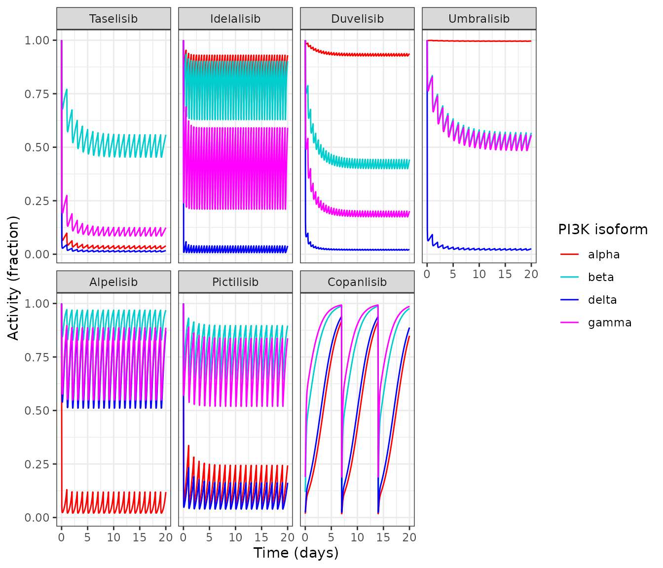
Replicates Figure 2 of Gadkar et al. (2022): normalized mucosal PI3K pathway activity (alpha red, beta cyan, gamma magenta, delta blue).
Table 2 of the paper puts each drug’s average alpha and delta inhibition into a category. The table below computes the mean inhibition over the third week (days 14 to 21) and checks it against those categories.
inh <- act |>
  dplyr::filter(time >= 14 * 24) |>
  dplyr::group_by(drug) |>
  dplyr::summarise(alpha_inh = 100 * (1 - mean(alpha)), delta_inh = 100 * (1 - mean(delta))) |>
  dplyr::mutate(drug = factor(drug, levels = drugs$drug)) |>
  dplyr::arrange(drug)
paper <- data.frame(
  drug = drugs$drug,
  alpha_paper = c(
    "Strong (>90%)", "Weak (10-25%)", "Weak (~5%)", "Negligible (~0%)",
    "Strong (>90%)", "Strong (75-90%)", "Strong->weak (90->15%)"
  ),
  delta_paper = c(
    "Strong (>90%)", "Strong (>90%)", "Strong (>90%)", "Strong (>90%)",
    "Mod/weak (15-55%)", "Strong (80-95%)", "Strong->weak (90->15%)"
  )
)
inh |>
  dplyr::mutate(drug = as.character(drug)) |>
  dplyr::left_join(paper, by = "drug") |>
  dplyr::mutate(alpha_inh = round(alpha_inh, 1), delta_inh = round(delta_inh, 1)) |>
  dplyr::rename(
    "Drug" = drug, "Mean alpha inhibition (%)" = alpha_inh, "Mean delta inhibition (%)" = delta_inh,
    "Paper alpha category" = alpha_paper, "Paper delta category" = delta_paper
  ) |>
knitr::kable(caption = "Mean mucosal inhibition over days 14-21 versus Table 2 of the paper.")| Drug | Mean alpha inhibition (%) | Mean delta inhibition (%) | Paper alpha category | Paper delta category |
|---|---|---|---|---|
| Taselisib | 96.8 | 98.6 | Strong (>90%) | Strong (>90%) |
| Idelalisib | 15.7 | 97.9 | Weak (10-25%) | Strong (>90%) |
| Duvelisib | 6.9 | 97.9 | Weak (~5%) | Strong (>90%) |
| Umbralisib | 0.4 | 97.8 | Negligible (~0%) | Strong (>90%) |
| Alpelisib | 94.7 | 30.9 | Strong (>90%) | Mod/weak (15-55%) |
| Pictilisib | 85.9 | 90.9 | Strong (75-90%) | Strong (80-95%) |
| Copanlisib | 56.4 | 50.1 | Strong->weak (90->15%) | Strong->weak (90->15%) |
# Deterministic (no IIV): the inhibition follows from PK and IC50 alone.
# The ranges below are the paper's Table 2 categories; for the "~"
# categories they are widened to +/- 5 points around the stated value.
# Copanlisib's category (strong -> weak, 90 -> 15%) describes the swing
# between a weekly dose and the end of that week, checked separately below.
g <- function(d, col) inh[[col]][inh$drug == d]
stopifnot(
  g("Taselisib", "alpha_inh") > 90, g("Taselisib", "delta_inh") > 90,
  g("Idelalisib", "alpha_inh") > 10, g("Idelalisib", "alpha_inh") < 25, g("Idelalisib", "delta_inh") > 90,
  g("Duvelisib", "alpha_inh") < 10, g("Duvelisib", "delta_inh") > 90,
  g("Umbralisib", "alpha_inh") < 5, g("Umbralisib", "delta_inh") > 90,
  g("Alpelisib", "alpha_inh") > 90, g("Alpelisib", "delta_inh") > 15, g("Alpelisib", "delta_inh") < 55,
  g("Pictilisib", "alpha_inh") > 75, g("Pictilisib", "alpha_inh") < 90,
  g("Pictilisib", "delta_inh") > 80, g("Pictilisib", "delta_inh") < 95
)

# Copanlisib: the week after the day-14 dose (days 14-20).
cop <- act |> dplyr::filter(drug == "Copanlisib", time >= 14 * 24, time <= 20 * 24)
cop_swing <- c(
  alpha_peak_inh = 100 * (1 - min(cop$alpha)), alpha_trough_inh = 100 * (1 - max(cop$alpha)),
  delta_peak_inh = 100 * (1 - min(cop$delta)), delta_trough_inh = 100 * (1 - max(cop$delta))
)
round(cop_swing, 1)
#>   alpha_peak_inh alpha_trough_inh   delta_peak_inh delta_trough_inh
#>             98.2             15.1             97.5             11.2
stopifnot(
  cop_swing[["alpha_peak_inh"]] > 85, cop_swing[["alpha_trough_inh"]] < 20,
  cop_swing[["delta_peak_inh"]] > 85, cop_swing[["delta_trough_inh"]] < 20
)
Replicate Figure 4a and 4d: IC50 sensitivity for taselisib
The paper raises the taselisib alpha IC50 (nominal 0.29 nM) and delta IC50 (nominal 0.12 nM) 10-, 30- and 100-fold. It reports that alpha inhibition falls “from greater than 95% to ~20% on average” and delta inhibition “from greater than 95% to ~40%” at 100-fold.
tas <- drugs[drugs$drug == "Taselisib", ]
sens <- dplyr::bind_rows(lapply(c(1, 10, 30, 100), function(f) {
  dplyr::bind_rows(lapply(c("alpha", "delta"), function(iso) {
    p <- drug_params(tas)
    nm <- if (iso == "alpha") "lic50_pi3ka" else "lic50_pi3kd"
    p[[nm]] <- p[[nm]] + log(f)
    s <- rxode2::rxSolve(mod, drug_events(tas, 21, obs20), params = p, returnType = "data.frame")
    data.frame(
      fold = f, isoform = iso, time = s$time,
      activity = if (iso == "alpha") s$PI3Ka_act else s$PI3Kd_act
    )
  }))
}))
ggplot(sens, aes(time / 24, activity, colour = factor(fold))) +
  geom_line() +
  facet_wrap(~isoform, labeller = labeller(isoform = c(alpha = "PI3K-alpha (Fig 4a)", delta = "PI3K-delta (Fig 4d)"))) +
  labs(x = "Time (days)", y = "Activity (fraction)", colour = "IC50 fold") +
  theme_bw()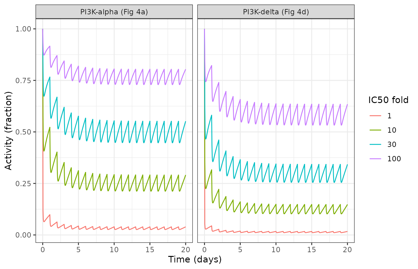
sens_inh <- sens |>
  dplyr::filter(time >= 14 * 24) |>
  dplyr::group_by(isoform, fold) |>
  dplyr::summarise(inhibition = 100 * (1 - mean(activity)), .groups = "drop")
knitr::kable(sens_inh, digits = 1, caption = "Mean inhibition (%) over days 14-21 by IC50 fold.")| isoform | fold | inhibition |
|---|---|---|
| alpha | 1 | 96.8 |
| alpha | 10 | 75.2 |
| alpha | 30 | 50.4 |
| alpha | 100 | 23.4 |
| delta | 1 | 98.6 |
| delta | 10 | 87.7 |
| delta | 30 | 70.5 |
| delta | 100 | 41.9 |
inh_at <- function(iso, f) sens_inh$inhibition[sens_inh$isoform == iso & sens_inh$fold == f]
stopifnot(
  inh_at("alpha", 1) > 95, inh_at("delta", 1) > 95,
  abs(inh_at("alpha", 100) - 20) < 5,
  abs(inh_at("delta", 100) - 40) < 5
)
Replicates Figure 4a and 4d of Gadkar et al. (2022).
Replicate Figure 6a: taselisib dosing holidays
d42 <- seq(0, 41) * 24
regimens <- list(
  "Daily" = d42,
  "5 days on, 2 off" = d42[(d42 / 24) %% 7 < 5],
  "14 days on, 7 off" = d42[(d42 / 24) %% 21 < 14]
)
hol <- dplyr::bind_rows(lapply(names(regimens), function(r) {
  ev <- rxode2::et(amt = tas$amt, time = regimens[[r]], cmt = "depot", rate = -2) |>
    rxode2::et(seq(0, 42 * 24, by = 1))
  s <- rxode2::rxSolve(mod, ev, params = drug_params(tas), returnType = "data.frame")
  data.frame(
    regimen = r, time = s$time,
    alpha = s$PI3Ka_act, beta = s$PI3Kb_act, gamma = s$PI3Kg_act, delta = s$PI3Kd_act
  )
}))
hol |>
  tidyr::pivot_longer(alpha:delta, names_to = "isoform", values_to = "activity") |>
  dplyr::mutate(regimen = factor(regimen, levels = names(regimens))) |>
  ggplot(aes(time / 24, activity, colour = regimen)) +
  geom_line() +
  facet_wrap(~isoform) +
  labs(x = "Time (days)", y = "Activity (fraction)", colour = "Regimen") +
  theme_bw()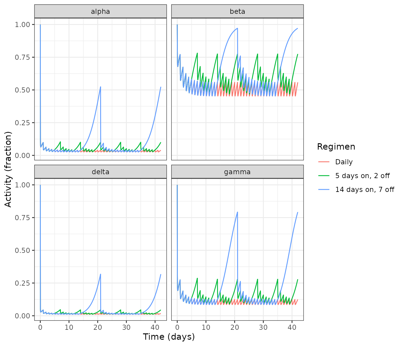
Replicates Figure 6a of Gadkar et al. (2022). As the paper notes, the alpha, gamma and delta activities do not return to 1 even during the 7-day holiday.
holiday <- hol |>
  dplyr::filter(regimen == "14 days on, 7 off", time > 14 * 24, time <= 21 * 24)
c(max_alpha = max(holiday$alpha), max_gamma = max(holiday$gamma), max_delta = max(holiday$delta))
#> max_alpha max_gamma max_delta
#> 0.5243836 0.7923789 0.3180844
stopifnot(max(holiday$alpha) < 1, max(holiday$gamma) < 1, max(holiday$delta) < 1)
Replicate Figure S1: response to an acute epithelial injury
Figure S1 shows the response to an acute epithelial injury given on
day 10, using the deposited dose Epi_activation_single (500
units into Activating_Event). Neutrophils, APCs and the GI
risk score rise and then resolve, “within 20-30 days consistent with
chemically induced colitis in preclinical models”.
ev_inj <- rxode2::et(amt = 500, time = 240, cmt = "Activating_Event", rate = -2) |>
  rxode2::et(seq(0, 70 * 24, by = 4))
inj <- rxode2::rxSolve(mod, ev_inj, returnType = "data.frame")
inj |>
  dplyr::select(time, Epithelial_Quality, GI_Risk_Score, APC_act, Neutrophils) |>
  tidyr::pivot_longer(-time) |>
  ggplot(aes(time / 24, value)) +
  geom_line() +
  facet_wrap(~name, scales = "free_y") +
  labs(x = "Time (days)", y = NULL) +
  theme_bw()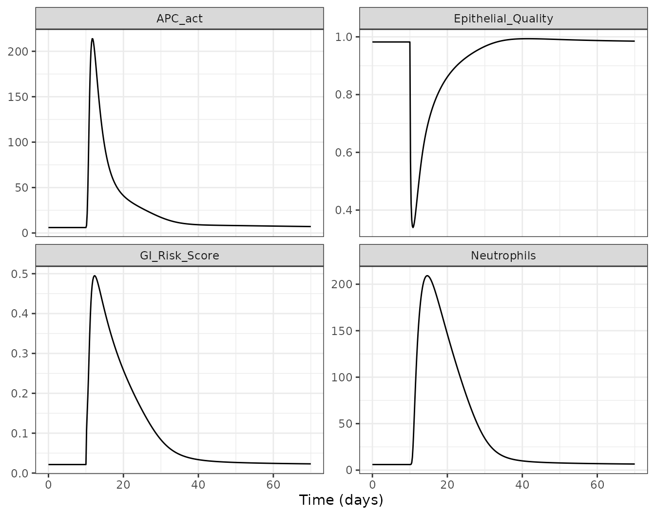
# Remaining excursion above the pre-injury level, as a fraction of the peak
# excursion, 30 days after the injury (day 40).
excursion <- function(x) (x[inj$time == 40 * 24] - x[1]) / (max(x) - x[1])
res_s1 <- c(
  peak_GI = max(inj$GI_Risk_Score),
  peak_neutrophils = max(inj$Neutrophils),
  GI_left_day40 = excursion(inj$GI_Risk_Score),
  APC_left_day40 = excursion(inj$APC_act),
  neutrophils_left_day40 = excursion(inj$Neutrophils)
)
signif(res_s1, 3)
#>                peak_GI       peak_neutrophils          GI_left_day40
#>                 0.4950               209.0000                 0.0259
#>         APC_left_day40 neutrophils_left_day40
#>                 0.0149                 0.0194
# Deterministic. The injury must produce a real transient (the GI risk
# score rises more than 10-fold), and less than 5% of each excursion may
# remain 30 days later (the paper: resolved within 20-30 days).
stopifnot(
  res_s1[["peak_GI"]] > 10 * inj$GI_Risk_Score[1],
  res_s1[["GI_left_day40"]] < 0.05,
  res_s1[["APC_left_day40"]] < 0.05,
  res_s1[["neutrophils_left_day40"]] < 0.05
)
In the baseline virtual patient, almost all of the inflammation resolves 26-30 days after the injury. A slow tail in the APC and T-cell densities takes several more weeks to return fully to baseline.
Replicates Figure S1 of Gadkar et al. (2022) for the baseline virtual patient. The paper plots the VPop mean and 5-95% band.
Baseline virtual patient on taselisib
The time course of one virtual patient on taselisib 4 mg once daily (compare Figure S8 for the VPop). The baseline virtual patient is a patient who does not develop diarrhea or colitis.
obs240 <- seq(0, 240 * 24, by = 6)
vp0 <- rxode2::rxSolve(mod, drug_events(tas, 240, obs240), params = drug_params(tas), returnType = "data.frame")
vp0 |>
  dplyr::select(time, Epithelial_Quality, GI_Risk_Score, APC_act, Neutrophils, T_Eff_act, RISK) |>
  tidyr::pivot_longer(-time) |>
  ggplot(aes(time / 24, value)) +
  geom_line() +
  facet_wrap(~name, scales = "free_y") +
  labs(x = "Time (days)", y = NULL) +
  theme_bw()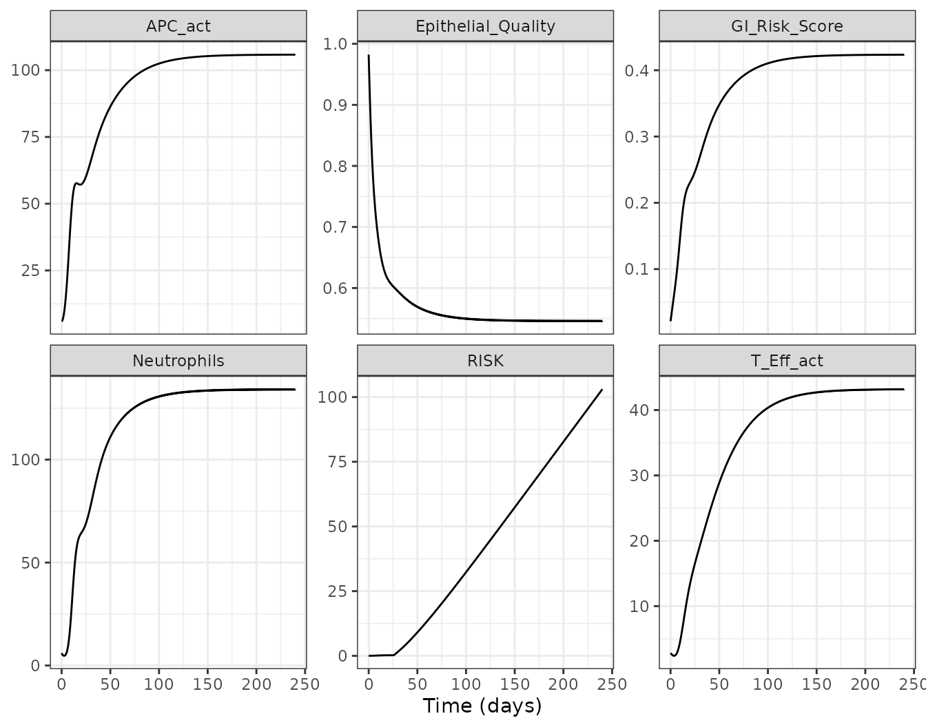
c(max_GI_Risk_Score = max(vp0$GI_Risk_Score), max_RISK = max(vp0$RISK))
#> max_GI_Risk_Score          max_RISK
#>          0.423543        103.045345
# Deterministic: the baseline virtual patient stays below both onset
# criteria (diarrhea GI > 0.6, colitis RISK > 200) under taselisib.
stopifnot(max(vp0$GI_Risk_Score) < 0.6, max(vp0$RISK) < 200)
Reproduction of the virtual-population incidences
The paper’s headline numbers are prevalence-weighted incidences across the 704-patient VPop. These are computed as follows:
- Run two 240-day drug-free run-ins.
- Dose for 240 days.
- Count diarrhea when
max(GI_Risk_Score) > 0.6and colitis whenmax(RISK) > 200.
On 2026-10-01 the maintainers re-simulated the authors’ deposited
VPOP.mat (88 parameters x 704 weighted patients) with the
equations and parameters in this model file. The results are below. They
are not recomputed at render time because the VPop is not distributed
with the package.
| Scenario | Paper diarrhea | Re-simulated diarrhea | Paper colitis | Re-simulated colitis |
|---|---|---|---|---|
| Taselisib 4 mg QD (Tables 2, 3) | 52% | 51.9% | 10.2% | 10.2% |
| Idelalisib 150 mg BID (Table 2) | – | 40.1% | 9.5% | 9.5% |
| Duvelisib 25 mg BID (Table 2) | – | 29.7% | 11.4% | 11.4% |
| Umbralisib 800 mg QD (Table 2) | – | 40.2% | 1.1% | 1.1% |
| Alpelisib 300 mg QD (Table 2) | – | 31.7% | 2.4% | 2.4% |
| Pictilisib 340 mg QD (Table 2) | – | 71.1% | 16.3% | 16.3% |
| Copanlisib 60 mg IV d1/8/15 q28d (Table 2) | – | 22.2% | 1.5% | 1.5% |
| Taselisib 5 days on, 2 off (Table 3) | 53% | 52.4% | 15% | 14.9% |
| Taselisib 14 days on, 7 off (Table 3) | 58% | 56.5% | 15% | 14.3% |
| Taselisib, alpha IC50 x100 (Figure 4b, c) | 27% | 26.7% | 7% | 6.4% |
| Taselisib, delta IC50 x100 (Figure 4e, f) | 18% | 17.5% | 3% | 2.5% |
All seven Table 2 colitis incidences reproduce to the printed decimal. Two of the 704 virtual patients could not be integrated by LSODA on the copanlisib schedule; they are counted as event-free. The small differences on the dosing-holiday regimens are consistent with the exact on/off day boundaries, which the deposit does not include.
PKNCA validation of the PK layer
The paper reports no NCA. The PK layer is therefore checked against
its own closed form. At steady state, the AUC over one dosing interval
equals F * Dose / CL, so 1000 * Dose / CL in
ng*h/mL with F = 1. The check uses each oral regimen after 28 days of
dosing, which is at least 11 half-lives for the slowest drug
(umbralisib).
oral <- drugs[drugs$route == "oral", ]
conc <- dplyr::bind_rows(lapply(seq_len(nrow(oral)), function(i) {
  d <- oral[i, ]
  t0 <- 28 * 24
  obs <- t0 + seq(0, d$ii, by = 0.05)
  ev <- rxode2::et(amt = d$amt, ii = d$ii, addl = (t0 + d$ii) / d$ii, cmt = "depot", rate = -2) |>
    rxode2::et(obs)
  s <- rxode2::rxSolve(mod, ev, params = drug_params(d), returnType = "data.frame", rtol = 1e-10, atol = 1e-12)
  data.frame(id = 1L, treatment = d$drug, time = s$time - t0, Cc = s$Cc)
}))
conc <- conc |>
  dplyr::filter(!is.na(Cc)) |>
  dplyr::mutate(Cc = pmax(Cc, 0))
dose_df <- data.frame(id = 1L, treatment = oral$drug, time = 0, amt = oral$amt)
intervals <- data.frame(
  start = 0, end = oral$ii, treatment = oral$drug,
  auclast = TRUE, cmax = TRUE, tmax = TRUE, cmin = TRUE
)
nca <- PKNCA::pk.nca(PKNCA::PKNCAdata(
  PKNCA::PKNCAconc(conc, Cc ~ time | treatment + id),
  PKNCA::PKNCAdose(dose_df, amt ~ time | treatment + id),
  intervals = intervals
))
res <- as.data.frame(nca$result) |>
  dplyr::select(treatment, PPTESTCD, PPORRES) |>
  tidyr::pivot_wider(names_from = PPTESTCD, values_from = PPORRES) |>
  dplyr::left_join(dplyr::transmute(oral, treatment = drug, auc_closed = 1000 * amt / cl), by = "treatment") |>
  dplyr::mutate(pct_diff = 100 * (auclast / auc_closed - 1))
res |>
  dplyr::rename(
    "Drug" = treatment, "Cmax,ss (ng/mL)" = cmax, "Tmax (h)" = tmax, "Cmin,ss (ng/mL)" = cmin,
    "AUCtau,ss PKNCA (ng*h/mL)" = auclast, "Dose/CL (ng*h/mL)" = auc_closed, "Difference (%)" = pct_diff
  ) |>
knitr::kable(digits = 3, caption = "Steady-state NCA of the PK layer versus the closed-form AUC.")| Drug | AUCtau,ss PKNCA (ng*h/mL) | Cmax,ss (ng/mL) | Cmin,ss (ng/mL) | Tmax (h) | Dose/CL (ng*h/mL) | Difference (%) |
|---|---|---|---|---|---|---|
| Taselisib | 799.999 | 40.256 | 26.289 | 3.55 | 800.00 | 0.000 |
| Idelalisib | 10080.586 | 1771.900 | 312.280 | 1.65 | 10080.65 | -0.001 |
| Duvelisib | 4999.992 | 448.206 | 374.152 | 3.00 | 5000.00 | 0.000 |
| Umbralisib | 91927.488 | 4366.768 | 3253.380 | 3.60 | 91954.02 | -0.029 |
| Alpelisib | 26086.922 | 2123.076 | 312.208 | 3.45 | 26086.96 | 0.000 |
| Pictilisib | 9964.820 | 819.106 | 169.354 | 1.75 | 9964.83 | 0.000 |
Assumptions and deviations
-
Default drug and virtual patient. The packaged
parameters are the deposited baseline virtual patient
VP0 (baseline VP)with taselisib PK and potency, which is the variant the deposited project applies by default. Other drugs are simulated by overriding the 11 drug parameters (seedrug_params()above andpopulation$notes). - Virtual population not carried. The 704 prevalence-weighted virtual patients are a non-parametric set, not an IIV distribution. The model is deterministic and has no residual error, because the paper fits none.
- Initial conditions. The deposit starts from the Table S1 cell densities with no epithelium and runs two 240-day drug-free run-ins before each treatment. The packaged initial conditions are the converged end of that run-in for the baseline virtual patient. If mechanistic parameters are changed, simulate a drug-free run-in (as the reproduction above did) before dosing.
-
Colitis threshold. Table 1 defines colitis onset as
the AUC of the GI risk score crossing 120 normalized-units-day. The
deposited code instead tests the state
RISK, which accumulatesk_healing * GIper hour and heals while GI is below 0.25, against- Only the deposited criterion reproduces Tables 2 and 3, so it is used here.
- Baseline GI risk score. Table S1 lists 0.23, but the model’s steady state is 0.021 (see the steady-state section).
- IC50 units and Table S3. The deposited IC50s are unbound ng/mL. For most drugs they equal the Table S3 nM values times the molecular weight. The taselisib beta IC50 of 4 ng/mL corresponds to the footnoted “30x relative selectivity” (0.29 x 30 = 8.7 nM), not to the 0.9 nM printed in the table. Pictilisib’s deposited IC50s do not follow Table S3 by a single factor. The deposited values, which generate the published results, are used throughout.
-
Collapsed activity rules. The deposit computes the
same isoform activity separately for each cell type,
e.g.
PI3Ka_EC,PI3Ka_APCandPI3Ka_T_Eff. These are identical expressions of the mucosal concentration, so the model carries one activity per isoform in the mucosa (PI3Ka_actand so on) and two in blood (PI3Kg_act_circandPI3Kd_act_circ). The deposited rulePI3Kg_Neutroand thePI3K_Inh_Tissue_SSaverage feed no rate and are omitted. -
Unused deposited parameters. Twelve parameters in
Parameters.xlsxappear in no rate law or rule of the deposit. They describe an immature-epithelial-cell pool and alternative epithelial-quality weights that are not part of the final model, and they are omitted:Epi_imm_qual_weight,Epi_Cell_act_weight,Epi_quies_qual_weight,Inflam_Colitis_w,Epi_imm_diff_rate_k,PI3Ka_ECimm_diff_EC50,PI3Ka_ECimm_diff_Emax,Epi_proliferation_rate_k,PI3Ka_ECimm_apop_IC50,PI3Ka_ECimm_apop_Imax,Epi_imm_apoptosis_rate_kandEpi_act_rate_k. -
Oral input. Deposited oral doses enter the gut
compartment as a 0.1-h zero-order input after a drug-specific lag. Use
rate = -2on oral dose records so the modelled duration is applied. Copanlisib is an IV bolus intocentral. -
Acute-injury timing. The deposited
Epi_activation_singledose starts at time 10. Figure S1 places the injury on day 10, so the replication doses at 240 h.