Acute urinary retention or BPH surgery: tamsulosin, dutasteride and combination (D'Agate 2021) • nlmixr2lib

Model and source

ui <- rxode2::rxode(readModelDb("DAgate_2021_bph_aurs_mbma"))

Citation: D’Agate S, Chavan C, Manyak M, Palacios-Moreno JM, Oelke M, Michel MC, Roehrborn CG, Della Pasqua O. Model-based meta-analysis of the time to first acute urinary retention or benign prostatic hyperplasia-related surgery in patients with moderate or severe symptoms. Br J Clin Pharmacol. 2021;87:2777-2789. doi:10.1111/bcp.14682. Hazard form from Methods 2.3 (Equations 2 and 3, the exponential density lambda * exp(-lambda * t)); covariate centring at the median from Results 3.3; parameter values from Table 3; centring medians from Table 2. The Supporting Information (BCP-87-2777-s001) contains the survival-function definitions and Figures S1-S3 only; the control stream the Methods refer to is not part of the deposit.
Article: https://doi.org/10.1111/bcp.14682

D’Agate 2021 is an individual-patient-data model-based meta-analysis of the time to the first episode of acute urinary retention or BPH-related surgery (AUR/S) in men with moderate or severe lower urinary tract symptoms due to benign prostatic hyperplasia. The data are the same six phase III/IV dutasteride trials (ARIA3001, ARIA3002, ARI40002, CombAT, CONDUCT, ARIB3003) that D’Agate 2020 used for its IPSS drug-disease model (Br J Clin Pharmacol 2020;86:1585-1599, doi:10.1111/bcp.14268).

Exponential, Gompertz and Weibull densities were compared and the exponential (constant) hazard was retained (Methods 2.3, Results 3.3). Baseline covariates and treatment act proportionally on the hazard (Equations 2 and 3), with the continuous covariates centred at their pooled medians (Results 3.3):

$h = \lambda \cdot \exp\Big(\sum_k \beta_k (x_k - \tilde{x}_k)\Big) \cdot HR_{treatment},\qquad S(t) = e^{-h t}$

The model integrates d/dt(cumhaz) <- hazard and reports sur = exp(-cumhaz), the probability of being free of AUR/S at time t (days).

Population

str(ui$population)
#> List of 11
#>  $ species       : chr "human"
#>  $ n_subjects    : int 9832
#>  $ n_studies     : int 6
#>  $ age_range     : chr "47-94 years (median 66, mean 66.2)"
#>  $ weight_range  : chr "37-179 kg (median 82, mean 83.2)"
#>  $ sex_female_pct: num 0
#>  $ race_ethnicity: chr "white 9268, black 229, Hispanic 276, Asian 374 (Table 2)"
#>  $ disease_state : chr "Men with moderate or severe LUTS due to BPH at risk of progression; baseline IPSS median 16 (range 1-35), PSA m"| __truncated__
#>  $ dose_range    : chr "Placebo (n = 2158, 2 y); watchful waiting with protocol-defined tamsulosin initiation (n = 373); tamsulosin 0.4"| __truncated__
#>  $ regions       : chr "multinational"
#>  $ notes         : chr "Studies ARIA3001, ARIA3002, ARI40002, CombAT, CONDUCT and ARIB3003 (Table 1). Of 10,238 pooled patients, 402 (2"| __truncated__

Table 2 of the paper summarises the pooled population: men aged 47-94 years (median 66), body weight median 82 kg, baseline IPSS median 16 (range 1-35), PSA median 3.4 ng/mL (0.6-23.2), prostate volume median 48.5 mL (16.6-296.9), maximum urinary flow median 10.2 mL/s (2.2-36.2), predominantly white (9268 white, 229 black, 276 Hispanic, 374 Asian). 2158 men received placebo for 2 years, 373 watchful waiting (CONDUCT), 1611 tamsulosin 0.4 mg (CombAT), 3790 dutasteride 0.5 mg and 2143 tamsulosin-dutasteride combination therapy for up to 4 years. The final data set holds 9832 patients once 402 CONDUCT step-up and ARI40002 switch patients are excluded (Methods 2.2, Figure 1).

Source trace

Quantity	Model name	Value	Source
Hazard form (exponential, proportional covariates)	`hazard`	Eq. 3; density $\lambda e^{-\lambda t}$	Methods 2.3; Results 3.3
Survival and cumulative hazard	`cumhaz`, `sur`	$S = e^{-H}$ , $H = \int h$	Supporting Information, ‘Parameterisation of the hazard function’
Baseline hazard	`llam_haz`	7.78 per 100,000 per day = 7.78e-5 /day	Table 3
Baseline IPSS HR	`e_ipss_bl_haz`	log(1.04), centred at 16	Table 3; median Table 2
Baseline PSA HR	`e_psa_bl_haz`	log(1.08) per ng/mL, centred at 3.4	Table 3; median Table 2
Baseline prostate volume HR	`e_prostate_vol_bl_haz`	log(1.01) per mL, centred at 48.5	Table 3; median Table 2
Baseline Qmax HR	`e_qmax_bl_haz`	log(0.91) per mL/s, centred at 10.2	Table 3; median Table 2
Tamsulosin HR	`e_trt_tamsulosin_haz`	log(1), fixed	Table 3; Results 3.3
Dutasteride HR	`e_trt_dutasteride_haz`	log(0.432)	Table 3
Combination HR	`e_trt_tamsulosin_dutasteride_haz`	log(0.336)	Table 3
Residual error	`addSd`	0.001, fixed placeholder	not from the source

Structural checks

The baseline hazard is the published 2.84% per year

Results 3.3 states that the baseline hazard corresponds to an incidence of 2.84% events per year, and Figures 4-6 use 2.84% as the colour midpoint.

lam <- exp(ui$theta[["llam_haz"]])
annual_pct <- 100 * lam * 365.25
annual_pct
#> [1] 2.841645
stopifnot(abs(annual_pct - 2.84) < 0.005)

The solved survival matches the closed form

The hazard is constant in time for a given patient, so $S(t) = e^{-h t}$ exactly. Both sides use the same parameters and covariates, so the difference is pure integration error and a tight bound is correct.

arms <- tibble::tribble(
  ~arm,             ~TRT_TAMSULOSIN, ~TRT_DUTASTERIDE, ~TRT_TAMSULOSIN_DUTASTERIDE,
  "Placebo",        0,               0,                0,
  "Tamsulosin",     1,               0,                0,
  "Dutasteride",    0,               1,                0,
  "Combination",    0,               0,                1
)
typical <- arms |>
  mutate(id = row_number(), IPSS_BL = 16, PSA_BL = 3.4,
         PROSTATE_VOL_BL = 48.5, QMAX_BL = 10.2)

obs_times <- seq(0, 48 * 30.4375, length.out = 49)
ev_typ <- typical |>
  select(id) |>
  tidyr::crossing(time = obs_times) |>
  mutate(evid = 0, cmt = "cumhaz", amt = 0) |>
  left_join(typical, by = "id")

sim_typ <- rxode2::rxSolve(ui, events = ev_typ, keep = "arm",
                           returnType = "data.frame")
#> Warning: multi-subject simulation without without 'omega'

hr_trt <- c(Placebo = 1, Tamsulosin = 1, Dutasteride = 0.432, Combination = 0.336)
chk <- sim_typ |>
  mutate(closed = exp(-lam * hr_trt[arm] * time))
max_abs_err <- max(abs(chk$sur - chk$closed))
max_abs_err
#> [1] 1.110223e-16
stopifnot(max_abs_err < 1e-6)

ggplot(sim_typ, aes(time / 30.4375, 100 * sur, colour = arm)) +
  geom_line(linewidth = 0.8) +
  labs(x = "Time (months)", y = "AUR/S-free survival (%)", colour = NULL,
       title = "Typical patient at the pooled median covariates") +
  theme_bw()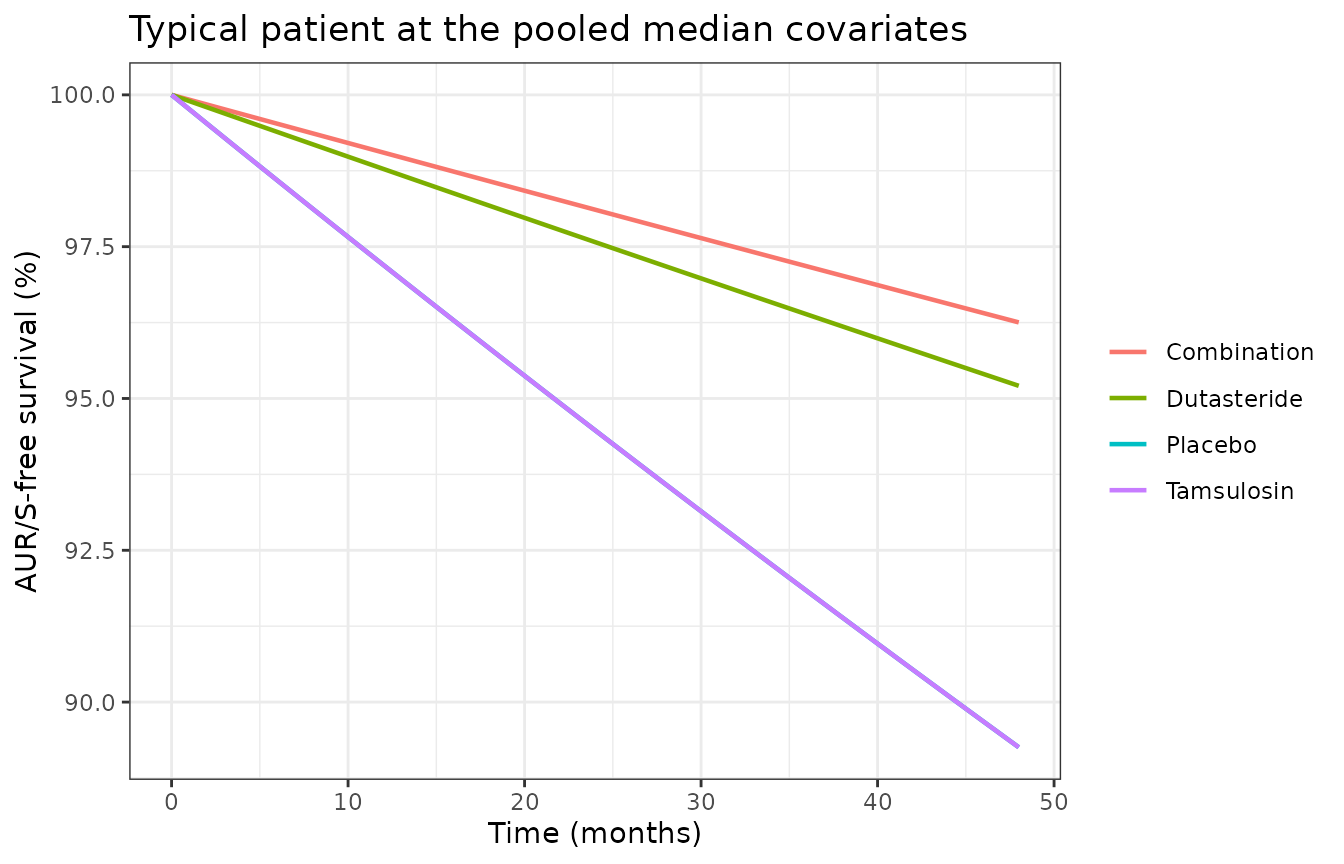

Replicate published figures

Heat maps of yearly AUR/S incidence (Figures 4-6)

Figures 4-6 print the model-predicted yearly incidence of AUR/S (%/yr) in each cell of a 5 x 5 grid of two baseline covariates, for mild, moderate and severe baseline symptoms and for each treatment. The maintainers transcribed the printed cell values. The figures do not say at which values they held the third covariate or at which IPSS they placed each severity band, so the absolute level of a cell cannot be reproduced. Ratios can be, because under proportional hazards those unstated values cancel:

Within a panel, each cell divided by the panel’s centre cell depends only on the two plotted covariates and their hazard ratios.
Across treatments, a dutasteride or combination cell divided by the placebo cell at the same position is the treatment hazard ratio.

Reading the rows confirms that the figures plot the hazard itself (100 * h * 365.25) rather than a one-year cumulative incidence 100 * (1 - exp(-h * 365.25)). The ratio between two columns is the same in the lowest and highest rows of a panel (for example Figure 5 severe placebo, 31.9 -> 96.6 mL: 2.20 -> 4.02 and 6.07 -> 11.09, both x1.83). A cumulative incidence would compress the ratio at the higher values.

# Rows are the y-axis values from the top of each panel; columns follow the
# x-axis from left to right.
read_panel <- function(txt, fig, trt, sev, yvar, yvals, xvar, xvals) {
  m <- as.matrix(utils::read.table(text = txt))
  dimnames(m) <- NULL
  tidyr::expand_grid(yi = seq_along(yvals), xi = seq_along(xvals)) |>
    mutate(figure = fig, treatment = trt, severity = sev,
           yvar = yvar, y = yvals[yi], xvar = xvar, x = xvals[xi],
           published = m[cbind(yi, xi)])
}
pv <- c(96.6, 61.8, 50.6, 39.4, 31.9)
psa <- c(1.6, 2.3, 3.5, 5.2, 8.2)
qmax <- c(16.3, 12.3, 10.5, 8.1, 5.4)
pv_x <- c(31.9, 39.4, 50.6, 61.8, 96.6)

heat <- bind_rows(
  # Figure 4: prostate volume (rows) x PSA (columns)
  read_panel("2.59 2.73 3 3.41 4.29
              1.87 1.98 2.17 2.47 3.1
              1.69 1.78 1.95 2.22 2.8
              1.52 1.61 1.76 2 2.52
              1.42 1.5 1.64 1.87 2.35", 4, "Placebo", "Mild", "PV", pv, "PSA", psa),
  read_panel("3.57 3.77 4.13 4.71 5.92
              2.58 2.73 2.99 3.4 4.28
              2.33 2.46 2.7 3.07 3.86
              2.1 2.22 2.43 2.77 3.48
              1.96 2.07 2.26 2.58 3.24", 4, "Placebo", "Moderate", "PV", pv, "PSA", psa),
  read_panel("5.9 6.23 6.82 7.77 9.78
              4.27 4.5 4.93 5.62 7.07
              3.85 4.06 4.45 5.07 6.37
              3.47 3.66 4.01 4.57 5.74
              3.23 3.41 3.74 4.26 5.36", 4, "Placebo", "Severe", "PV", pv, "PSA", psa),
  read_panel("1.54 1.63 1.79 2.03 2.56
              1.12 1.18 1.29 1.47 1.85
              1.01 1.06 1.16 1.33 1.67
              0.91 0.96 1.05 1.19 1.5
              0.85 0.89 0.98 1.11 1.4", 4, "Dutasteride", "Moderate", "PV", pv, "PSA", psa),
  read_panel("2.55 2.69 2.95 3.36 4.22
              1.84 1.94 2.13 2.43 3.05
              1.66 1.75 1.92 2.19 2.75
              1.5 1.58 1.73 1.97 2.48
              1.4 1.47 1.61 1.84 2.31", 4, "Dutasteride", "Severe", "PV", pv, "PSA", psa),
  read_panel("1.2 1.27 1.39 1.58 1.99
              0.87 0.92 1 1.14 1.44
              0.78 0.83 0.91 1.03 1.3
              0.71 0.74 0.82 0.93 1.17
              0.66 0.69 0.76 0.87 1.09", 4, "Combination", "Moderate", "PV", pv, "PSA", psa),
  read_panel("1.98 2.09 2.29 2.61 3.28
              1.43 1.51 1.66 1.89 2.38
              1.29 1.36 1.49 1.7 2.14
              1.16 1.23 1.35 1.53 1.93
              1.09 1.15 1.26 1.43 1.8", 4, "Combination", "Severe", "PV", pv, "PSA", psa),
  # Figure 5: Qmax (rows) x prostate volume (columns)
  read_panel("0.97 1.04 1.15 1.28 1.76
              1.41 1.51 1.67 1.86 2.57
              1.66 1.78 1.98 2.19 3.03
              2.08 2.23 2.47 2.74 3.79
              2.67 2.86 3.17 3.52 4.87", 5, "Placebo", "Mild", "QMAX", qmax, "PV", pv_x),
  read_panel("1.33 1.43 1.59 1.76 2.44
              1.94 2.08 2.31 2.56 3.54
              2.29 2.46 2.73 3.03 4.18
              2.86 3.07 3.41 3.78 5.23
              3.68 3.95 4.38 4.86 6.72", 5, "Placebo", "Moderate", "QMAX", qmax, "PV", pv_x),
  read_panel("2.2 2.36 2.62 2.91 4.02
              3.2 3.44 3.81 4.23 5.85
              3.78 4.06 4.5 5 6.91
              4.73 5.07 5.63 6.24 8.63
              6.07 6.51 7.23 8.02 11.09", 5, "Placebo", "Severe", "QMAX", qmax, "PV", pv_x),
  # Figure 6: Qmax (rows) x PSA (columns)
  read_panel("1 1.06 1.16 1.32 1.66
              1.46 1.54 1.68 1.92 2.41
              1.72 1.82 1.99 2.27 2.85
              2.15 2.27 2.49 2.83 3.56
              2.76 2.91 3.19 3.64 4.58", 6, "Placebo", "Mild", "QMAX", qmax, "PSA", psa),
  read_panel("1.38 1.46 1.6 1.82 2.29
              2.01 2.12 2.33 2.65 3.33
              2.37 2.51 2.75 3.13 3.93
              2.97 3.13 3.43 3.91 4.92
              3.81 4.02 4.41 5.02 6.32", 6, "Placebo", "Moderate", "QMAX", qmax, "PSA", psa),
  read_panel("2.28 2.41 2.64 3 3.78
              3.32 3.5 3.84 4.37 5.5
              3.92 4.14 4.53 5.16 6.5
              4.9 5.17 5.67 6.45 8.12
              6.29 6.64 7.28 8.29 10.43", 6, "Placebo", "Severe", "QMAX", qmax, "PSA", psa)
)

The model side is solved with rxode2 on the same grids. The covariate not on either axis is held at its median and IPSS at 16; these choices cancel in the ratios.

cells <- heat |>
  mutate(
    PSA_BL = case_when(xvar == "PSA" ~ x, TRUE ~ 3.4),
    PROSTATE_VOL_BL = case_when(yvar == "PV" ~ y, xvar == "PV" ~ x, TRUE ~ 48.5),
    QMAX_BL = case_when(yvar == "QMAX" ~ y, TRUE ~ 10.2),
    IPSS_BL = 16,
    TRT_TAMSULOSIN = 0,
    TRT_DUTASTERIDE = as.numeric(treatment == "Dutasteride"),
    TRT_TAMSULOSIN_DUTASTERIDE = as.numeric(treatment == "Combination"),
    id = row_number(), time = 0, evid = 0, cmt = "cumhaz", amt = 0
  )
sim_cells <- rxode2::rxSolve(ui, events = cells, returnType = "data.frame")
#> Warning: multi-subject simulation without without 'omega'
cells$model <- 100 * sim_cells$hazard * 365.25

centre <- cells |>
  filter(yi == 3, xi == 3) |>
  select(figure, treatment, severity, pub_ref = published, mod_ref = model)
within <- cells |>
  left_join(centre, by = c("figure", "treatment", "severity")) |>
  mutate(pub_ratio = published / pub_ref, mod_ratio = model / mod_ref,
         pct_diff = 100 * (mod_ratio / pub_ratio - 1))

within |>
  group_by(Figure = figure, Axes = paste(yvar, "x", xvar)) |>
  summarise(Cells = n(),
            `Median % diff` = round(median(pct_diff), 2),
            `Max abs % diff` = round(max(abs(pct_diff)), 2),
            .groups = "drop") |>
  knitr::kable(caption = "Within-panel ratios to the centre cell, model versus Figures 4-6.")

Within-panel ratios to the centre cell, model versus Figures 4-6.
Figure	Axes	Cells	Median % diff	Max abs % diff
4	PV x PSA	175	0.00	3.77
5	QMAX x PV	75	0.04	3.95
6	QMAX x PSA	75	0.05	1.06

The within-panel ratios reproduce the figures exactly along the PSA and Qmax axes, apart from the two-digit rounding of the printed cells. Along the prostate-volume axis the model’s gradient is a little steeper: the figures imply about 1.0094 per mL, inside the Table 3 95% CI of 1.007-1.012, whereas the model carries the printed 1.01. Relative to the 50.6 mL centre cell, the largest resulting difference (at 96.6 mL) is about 4%, which is the maximum in the table.

# Implied per-unit hazard ratio along each axis, from the corner cells of every
# placebo panel.
implied <- cells |>
  filter(treatment == "Placebo") |>
  group_by(figure, severity) |>
  summarise(
    x_hr = exp(log(published[yi == 3 & xi == 5] / published[yi == 3 & xi == 1]) /
                 (x[xi == 5][1] - x[xi == 1][1])),
    y_hr = exp(log(published[yi == 1 & xi == 3] / published[yi == 5 & xi == 3]) /
                 (y[yi == 1][1] - y[yi == 5][1])),
    xvar = xvar[1], yvar = yvar[1], .groups = "drop"
  )
implied_hr <- bind_rows(
  implied |> select(figure, severity, covariate = xvar, hr = x_hr),
  implied |> select(figure, severity, covariate = yvar, hr = y_hr)
) |>
  group_by(covariate) |>
  summarise(`Figures 4-6 implied HR per unit` = round(mean(hr), 4),
            .groups = "drop") |>
  mutate(`Table 3 HR` = c(PSA = 1.08, PV = 1.01, QMAX = 0.91)[covariate])
knitr::kable(implied_hr)

covariate	Figures 4-6 implied HR per unit	Table 3 HR
PSA	1.0795	1.08
PV	1.0094	1.01
QMAX	0.9112	0.91

stopifnot(
  # PSA and Qmax gradients: exact apart from two-digit rounding of the cells.
  with(filter(within, xvar != "PV", yvar != "PV"), max(abs(pct_diff))) < 2,
  # Prostate-volume gradient: printed HR 1.01 versus the ~1.0094 the figures
  # were drawn with, about 4% from the 50.6 mL centre cell to 96.6 mL.
  max(abs(within$pct_diff)) < 5,
  abs(implied_hr$`Figures 4-6 implied HR per unit`[implied_hr$covariate == "PSA"] - 1.08) < 0.002,
  abs(implied_hr$`Figures 4-6 implied HR per unit`[implied_hr$covariate == "QMAX"] - 0.91) < 0.002
)

The treatment hazard ratios are recovered exactly from the Figure 4 panels:

trt_ratio <- cells |>
  filter(figure == 4, severity != "Mild") |>
  select(severity, yi, xi, treatment, published) |>
  tidyr::pivot_wider(names_from = treatment, values_from = published) |>
  tidyr::pivot_longer(c(Dutasteride, Combination), names_to = "treatment",
                      values_to = "active") |>
  mutate(hr = active / Placebo)
trt_tab <- trt_ratio |>
  group_by(Treatment = treatment) |>
  summarise(`Figure 4 median ratio to placebo` = round(median(hr), 3),
            `Figure 4 ratio range` = paste(round(range(hr), 3), collapse = " - "),
            .groups = "drop") |>
  mutate(`Table 3 HR` = c(Dutasteride = 0.432, Combination = 0.336)[Treatment])
knitr::kable(trt_tab)

Treatment	Figure 4 median ratio to placebo	Figure 4 ratio range	Table 3 HR
Combination	0.336	0.333 - 0.338	0.336
Dutasteride	0.432	0.43 - 0.434	0.432

stopifnot(
  abs(median(trt_ratio$hr[trt_ratio$treatment == "Dutasteride"]) - 0.432) < 0.005,
  abs(median(trt_ratio$hr[trt_ratio$treatment == "Combination"]) - 0.336) < 0.005
)

The severity bands only move the level of a panel, and the IPSS values the authors used for them are not stated. At a hazard ratio of 1.04 per point, the panel-to-panel ratios correspond to these IPSS gaps:

sev_gap <- cells |>
  filter(treatment == "Placebo") |>
  group_by(figure, yi, xi) |>
  summarise(mild_to_moderate = log(published[severity == "Moderate"] /
                                     published[severity == "Mild"]) / log(1.04),
            moderate_to_severe = log(published[severity == "Severe"] /
                                       published[severity == "Moderate"]) / log(1.04),
            .groups = "drop")
round(c(mild_to_moderate = median(sev_gap$mild_to_moderate),
        moderate_to_severe = median(sev_gap$moderate_to_severe)), 1)
#>   mild_to_moderate moderate_to_severe 
#>                8.2               12.8

These gaps are consistent with representative scores of, for example, about 5, 13 and 26 points for the mild (0-7), moderate (8-19) and severe (20-35) bands.

cells |>
  filter(figure == 4) |>
  mutate(treatment = factor(treatment, c("Placebo", "Dutasteride", "Combination")),
         severity = factor(severity, c("Mild", "Moderate", "Severe"))) |>
  ggplot(aes(factor(x), factor(y), fill = model)) +
  geom_tile() +
  geom_text(aes(label = sprintf("%.2f", model)), size = 2.6) +
  facet_grid(severity ~ treatment) +
  scale_fill_gradient2(low = "green3", mid = "yellow", high = "red",
                       midpoint = 2.84, name = "Incidence\n(%/yr)") +
  labs(x = "Prostate-specific antigen (ng/mL)", y = "Prostate volume (mL)",
       title = "Model incidence at IPSS 16 and median Qmax (layout of Figure 4)") +
  theme_bw()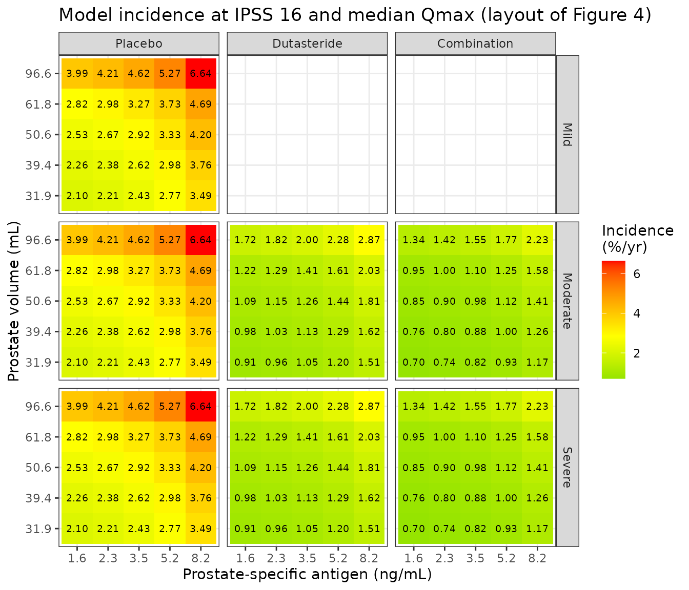

Survival by treatment (Figure 3)

Figure 3 is a visual predictive check of the Kaplan-Meier AUR/S-free survival by treatment arm. The trial populations behind each arm differ (tamsulosin monotherapy comes only from CombAT, which enrolled men with larger prostates and higher PSA, and placebo only from the 2-year dutasteride registration trials), and the per-arm covariate distributions are not published. The simulation below therefore gives every arm the same virtual cohort drawn from the pooled Table 2 distributions. It shows the treatment effect on a common population, not a reproduction of each arm’s observed curve.

Virtual cohort

IPSS is drawn from a normal distribution with the Table 2 mean and SD. PSA, prostate volume and Qmax are drawn from log-normal distributions with the Table 2 median and SD. All four are truncated to the Table 2 range, and the four covariates are drawn independently.

set.seed(2021)
n_per_arm <- 200

lnorm_sdlog <- function(median, sd) {
  stats::uniroot(function(s) median * exp(s^2 / 2) * sqrt(exp(s^2) - 1) - sd,
                 c(1e-3, 3))$root
}
# Truncation by rejection: values outside the Table 2 range are redrawn, not
# clamped to the limit (clamping would pile probability mass on the limits).
draw_truncated <- function(n, rdraw, lo, hi) {
  out <- numeric(0)
  while (length(out) < n) {
    x <- rdraw(n)
    out <- c(out, x[x >= lo & x <= hi])
  }
  out[seq_len(n)]
}
draw_lnorm <- function(n, median, sd, lo, hi) {
  sdlog <- lnorm_sdlog(median, sd)
  draw_truncated(n, function(m) stats::rlnorm(m, log(median), sdlog), lo, hi)
}
cohort <- tibble::tibble(
  pid = seq_len(n_per_arm),
  IPSS_BL = draw_truncated(
    n_per_arm, function(m) round(stats::rnorm(m, 16.48, 6.10)), 1, 35
  ),
  PSA_BL = draw_lnorm(n_per_arm, 3.4, 2.10, 0.6, 23.2),
  PROSTATE_VOL_BL = draw_lnorm(n_per_arm, 48.5, 23.0, 16.59, 296.89),
  QMAX_BL = draw_lnorm(n_per_arm, 10.2, 3.59, 2.2, 36.2)
)
summary(cohort[, -1])
#>     IPSS_BL          PSA_BL        PROSTATE_VOL_BL     QMAX_BL      
#>  Min.   : 3.00   Min.   : 0.7743   Min.   : 18.61   Min.   : 3.602  
#>  1st Qu.:12.00   1st Qu.: 2.3710   1st Qu.: 39.29   1st Qu.: 7.913  
#>  Median :16.00   Median : 3.5613   Median : 49.92   Median :10.132  
#>  Mean   :16.09   Mean   : 4.0928   Mean   : 55.87   Mean   :10.743  
#>  3rd Qu.:20.00   3rd Qu.: 5.2702   3rd Qu.: 67.75   3rd Qu.:12.761  
#>  Max.   :33.00   Max.   :16.7999   Max.   :207.25   Max.   :25.465

Simulation

subjects <- tidyr::crossing(arms, cohort) |>
  mutate(id = row_number())
ev_vpc <- subjects |>
  select(id) |>
  tidyr::crossing(time = seq(0, 48 * 30.4375, by = 30.4375)) |>
  mutate(evid = 0, cmt = "cumhaz", amt = 0) |>
  left_join(subjects, by = "id")
sim <- rxode2::rxSolve(ui, events = ev_vpc, keep = "arm",
                       returnType = "data.frame")
#> Warning: multi-subject simulation without without 'omega'

surv_arm <- sim |>
  group_by(arm, time) |>
  summarise(sur = mean(sur), .groups = "drop") |>
  mutate(arm = factor(arm, arms$arm))

# Structure of Figure 3 of D'Agate 2021: AUR/S-free survival by treatment.
ggplot(surv_arm, aes(time / 30.4375, 100 * sur)) +
  geom_line(colour = "blue", linewidth = 0.8) +
  facet_wrap(~arm) +
  coord_cartesian(ylim = c(86, 100)) +
  scale_x_continuous(breaks = seq(0, 48, by = 6)) +
  labs(x = "Time (months)", y = "Survival (%)",
       title = "Population-mean AUR/S-free survival, pooled Table 2 cohort") +
  theme_bw()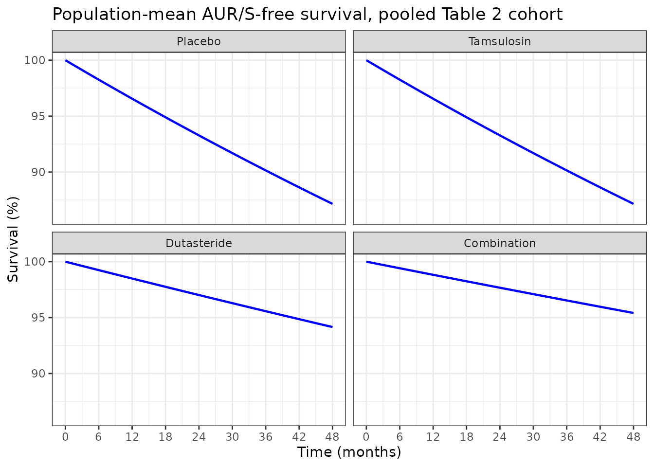

fig3 <- tibble::tribble(
  ~arm,          ~months, ~figure3_observed_pct,
  "Placebo",     24,      93,
  "Tamsulosin",  48,      87.5,
  "Dutasteride", 48,      94.3,
  "Combination", 48,      95.8
)
fig3_chk <- fig3 |>
  left_join(surv_arm |>
              mutate(months = round(time / 30.4375), arm = as.character(arm)),
            by = c("arm", "months"))
# Every arm is matched, and each model value is within 1 percentage point of
# the Figure 3 read-off (the covariates are drawn with base R's RNG and the
# model has no random effects, so these values do not depend on the rxode2
# build).
stopifnot(
  nrow(fig3_chk) == 4,
  !anyNA(fig3_chk$sur),
  all(abs(100 * fig3_chk$sur - fig3_chk$figure3_observed_pct) < 1)
)
fig3_chk |>
  transmute(Arm = arm, Months = months,
            `Figure 3 observed (%, read off the plot)` = figure3_observed_pct,
            `Model, pooled cohort (%)` = round(100 * sur, 1)) |>
  knitr::kable()

Arm	Months	Figure 3 observed (%, read off the plot)	Model, pooled cohort (%)
Placebo	24	93.0	93.3
Tamsulosin	48	87.5	87.2
Dutasteride	48	94.3	94.2
Combination	48	95.8	95.4

The model values fall within 1 percentage point of the observed Kaplan-Meier curves read off Figure 3. The tamsulosin arm ends lowest only because its follow-up runs to 48 months, twice that of the placebo arm. The two share one hazard (the tamsulosin hazard ratio is fixed to 1), so the model’s tamsulosin curve at 24 months equals its placebo curve. Because every arm here uses the same pooled cohort, the agreement is a plausibility check rather than a per-arm reproduction.

PKNCA validation

Not applicable. The model has no drug concentrations or dosing events. Treatment enters only as an arm indicator on the hazard, and the outputs are a hazard, a cumulative hazard and a survival probability. The closed-form survival check and the Figure 4-6 ratio gates above replace the NCA comparison.

Assumptions and deviations

Covariate centring. The paper states the centring in words only (Results 3.3, “starting from the median value of the covariate factor”). The control stream that Methods 2.3 says is in the Supporting Information is not part of the published deposit, which contains only the survival-function definitions and Figures S1-S3. The centring values are the pooled medians of Table 2 (IPSS 16, PSA 3.4 ng/mL, prostate volume 48.5 mL, Qmax 10.2 mL/s). The authors imputed missing values with study-level medians (Methods 2.2), so their fitted centring may differ slightly by study. With these medians and the Table 3 baseline hazard, a placebo patient at the medians has the published 2.84% per year.
Log-linear covariate form. Equation 2 defines each hazard ratio as $e^{\beta}$ per unit, so a patient 10 IPSS points above the median has $1.04^{10} = 1.48$ times the hazard. Results 3.3 describes this example informally as “40% higher”. The model follows the equation, and the Figure 4-6 cell ratios confirm the multiplicative form (for example the PSA gradient is 1.08 per ng/mL across the whole 1.6-8.2 ng/mL range).
Rounded hazard ratios. Table 3 prints the covariate hazard ratios to two decimals. The prostate-volume gradient in Figures 4-6 implies about 1.0094 per mL, so the published figures were drawn with an unrounded estimate. The model keeps the printed 1.01, which is inside the Table 3 95% CI of 1.007-1.012. The IPSS hazard ratio’s 95% CI of 1.022-1.050 is centred at 1.036, so the printed 1.04 is probably also rounded.
Tamsulosin. The effect was not significant and was fixed to a hazard ratio of 1 (Results 3.3). It is carried as a fixed zero log-hazard ratio so the arm indicator is explicit.
Watchful waiting. No effect could be estimated (“small sample size and very low number of events”, Results 3.3), and Table 3 has no row for it. A watchful-waiting patient therefore carries the placebo hazard. The indicator is documented under covariatesDataExcluded.
No variance components. As Methods 2.3 states, the time-to-event model has no between-subject, between-occasion or residual variability. The additive residual addSd = 0.001 on sur is a fixed placeholder, so that nlmixr2 accepts the model for simulation, and is not from the source.
Time unit. Table 3 gives the baseline hazard per day, so the model runs in days. Months in the plots are 30.4375 days, and years are 365.25 days.
Screened covariates. Age, race, weight, height, BMI, smoking, alcohol use, sexual activity, duration of BPH symptoms and time since BPH diagnosis were tested and not retained (Methods 2.3, Results 3.3). No estimates are published for them.
Virtual cohort. The distributional shapes (normal IPSS, log-normal PSA, prostate volume and Qmax) and their independence are assumptions. Table 2 gives only summary statistics, and Figure S3 shows no strong correlations among these four covariates.
Figure 3 values were read off the published plot by the maintainers to about 0.5 percentage points and are indicative only.