SARS-CoV-2 viral dynamic models (Agyeman 2022)
Source:vignettes/articles/Agyeman_2022_covid19_viral_dynamics.Rmd
Agyeman_2022_covid19_viral_dynamics.RmdModel and source
- Citation: Agyeman AA, You T, Chan PLS, Lonsdale DO, Hadjichrysanthou C, Mahungu T, Wey EQ, Lowe DM, Lipman MCI, Breuer J, Kloprogge F, Standing JF. Comparative assessment of viral dynamic models for SARS-CoV-2 for pharmacodynamic assessment in early treatment trials. Br J Clin Pharmacol. 2022;88(12):5428-5433. doi:10.1111/bcp.15518
- Article: Br J Clin Pharmacol 2022;88(12):5428-5433 (open access, PMC9538685); parameter estimates are in Supporting Information Tables S2 and S3.
Agyeman et al. compared four published viral dynamic model structures for SARS-CoV-2 when fitted to Phase-II-like viral load time courses: the slope-intercept exponential decay model (SI), the reduced target-cell-limited model (rTCL), the target-cell-limited model (TCL) and the TCL model with an eclipse phase (TCLE). Each structure was fitted separately to two datasets in nlmixr 2.0.6 (SAEM), so the paper reports eight independent fits. Each fit is a separate model in nlmixr2lib:
| Structure | Dataset A (Gastine 2021) | Dataset B (Neant 2021) |
|---|---|---|
| SI | Agyeman_2022_covid19_si_gastine |
Agyeman_2022_covid19_si_neant |
| rTCL | Agyeman_2022_covid19_rtcl_gastine |
Agyeman_2022_covid19_rtcl_neant |
| TCL | Agyeman_2022_covid19_tcl_gastine |
Agyeman_2022_covid19_tcl_neant |
| TCLE | Agyeman_2022_covid19_tcle_gastine |
Agyeman_2022_covid19_tcle_neant |
model_names <- tidyr::expand_grid(
  structure = c("SI", "rTCL", "TCL", "TCLE"),
  dataset = c("A", "B")
) |>
  mutate(
    name = paste0(
      "Agyeman_2022_covid19_", tolower(structure), "_",
      ifelse(dataset == "A", "gastine", "neant")
    )
  )
uis <- lapply(setNames(model_names$name, model_names$name), function(nm) {
  rxode2::rxode(readModelDb(nm))
})
Population
Dataset A comprises 252 patients with 747 viral load samples, compiled at the patient level by the systematic review and meta-analysis of Gastine et al. (2021). Most patients had mild disease (one death was reported). Agyeman et al. kept only untreated patients and upper-respiratory-tract samples.
Dataset B comprises 321 patients with 563 nasopharyngeal viral load samples from the prospective French COVID cohort analysed by Neant et al. (2021). All patients were hospitalised (conventional wards or intensive care), 78 died during follow-up, and patients received routine antiviral, antibiotic, antifungal or corticosteroid treatment.
Both datasets were limited to the first 14 days after symptom onset. Age, sex and other demographics are reported in the two source publications, not in Agyeman 2022. The same information is available programmatically:
str(readModelDb("Agyeman_2022_covid19_si_neant")()$population[
  c("species", "n_subjects", "n_observations", "disease_state")
])
#> List of 4
#>  $ species       : chr "human"
#>  $ n_subjects    : int 321
#>  $ n_observations: int 563
#>  $ disease_state : chr "COVID-19 (SARS-CoV-2 infection) requiring hospitalisation in conventional wards or intensive care units; 78 dea"| __truncated__
Source trace
Every ini() value carries an in-file comment naming its
source. The table collects them. Values are Table S2 (dataset A) and
Table S3 (dataset B) of the Supporting Information; initial conditions
are the footnote shared by both tables; incubation periods come from the
Results text and Figures S1 and S2.
| Parameter (unit) | SI A | rTCL A | TCL A | TCLE A | SI B | rTCL B | TCL B | TCLE B |
|---|---|---|---|---|---|---|---|---|
V(0) at symptom onset, lrbase (copies/mL) |
1.8e7 | 1.46e7 | - | - | 1.89e8 | 1.3e8 | - | - |
beta, lbeta ((copies/mL)^-1 day^-1) |
- | 5.0e-4 | 7.06e-4 | 7.76e-5 | - | 1.27e-3 | 1.54e-3 | 9.79e-5 |
delta, ldelta (1/day) |
0.56 | 0.56 | 1.84 | 0.69 | 0.85 | 0.80 | 0.74 | 0.81 |
rho, lrho (copies/mL/day per cell/mL) |
- | - | 0.28 | 2.96e3 | - | - | 0.29 | 2.84e3 |
c, lc (1/day) |
- | - | 0.64 | 11.6 | - | - | 0.93 | 2.62 |
gamma, lgamma (1/day) |
- | 1 (fixed) | - | - | - | 1 (fixed) | - | - |
k, lk (1/day) |
- | - | - | 9.23 | - | - | - | 8.87 |
f(0), f0
|
- | 1 (fixed) | - | - | - | 1 (fixed) | - | - |
T(0), lT0 (cells/mL) |
- | - | 1e8 | 1.3e5 | - | - | 1e8 | 1.3e5 |
I1(0), lI10 (cells/mL) |
- | - | - | 1/30 | - | - | - | 1/30 |
V(0) at infection, lV0 (copies/mL) |
- | - | 1 | 0.1 | - | - | 1 | 0.1 |
Incubation period, tinc (day) |
- | - | 0.5 | 0.5 | - | - | 1 | 1.5 |
| Equation | Source |
|---|---|
SI: d/dt(virus) = -delta * virus
|
Equation 1 |
rTCL: d/dt(target) = -beta * f * V;
d/dt(virus) = gamma * f * V - delta * V
|
Equation 2 |
| TCL: T, I, V system | Equation 3 (sign of the infection term in dI/dt corrected; see Assumptions) |
TCLE: T, I1, I2, V system, with virion loss
beta * T * V in dV/dt |
Equation 4 (sign of the infection term in dI1/dt corrected) |
| R0 = gamma / delta (SI, rTCL); rho beta T0 / (c delta) (TCL); rho beta T0 / (delta (c + beta T0)) (TCLE) | Equations 5, 6, 7 |
| L = 1 / delta | Equation 8 |
| IIV: log-normal on every estimated parameter; residual: additive on log viral load | Section 2.3 (magnitudes not reported) |
Known-answer check: R0 and duration of virus production
Tables S2 and S3 report the basic reproduction number R0 and the
duration of virus production L for every fit. Both are closed-form
functions of the estimated parameters (Equations 5 to 8), so recomputing
them from the packaged ini() values tests the transcription
of every rate constant and initial condition at once: a wrong exponent
on beta or rho moves R0 by an order of magnitude.
r0_l <- function(ui, structure) {
  th <- ui$theta
  delta <- exp(th[["ldelta"]])
  r0 <- switch(structure,
    SI = NA_real_,
    rTCL = exp(th[["lgamma"]]) / delta,
    TCL = exp(th[["lrho"]] + th[["lbeta"]] + th[["lT0"]]) /
      (exp(th[["lc"]]) * delta),
    TCLE = exp(th[["lrho"]] + th[["lbeta"]] + th[["lT0"]]) /
      (delta * (exp(th[["lc"]]) + exp(th[["lbeta"]] + th[["lT0"]])))
  )
  c(R0 = r0, L = 1 / delta)
}

reported <- tibble::tribble(
  ~structure, ~dataset, ~R0_paper, ~L_paper,
  "SI",   "A", NA,    1.79,
  "rTCL", "A", 1.79,  1.79,
  "TCL",  "A", 16787, 0.54,
  "TCLE", "A", 1995,  1.45,
  "SI",   "B", NA,    1.18,
  "rTCL", "B", 1.25,  1.25,
  "TCL",  "B", 64894, 1.35,
  "TCLE", "B", 2908,  1.23
)

chk_r0 <- model_names |>
  rowwise() |>
  mutate(
    R0_model = r0_l(uis[[name]], structure)[["R0"]],
    L_model = r0_l(uis[[name]], structure)[["L"]]
  ) |>
  ungroup() |>
  left_join(reported, by = c("structure", "dataset")) |>
  mutate(
    R0_pct_diff = 100 * (R0_model / R0_paper - 1),
    L_pct_diff = 100 * (L_model / L_paper - 1)
  )

chk_r0 |>
  select(structure, dataset, R0_paper, R0_model, R0_pct_diff,
         L_paper, L_model, L_pct_diff) |>
  dplyr::rename(
    "Structure" = structure, "Dataset" = dataset,
    "R0 (paper)" = R0_paper, "R0 (model)" = R0_model,
    "R0 diff (%)" = R0_pct_diff, "L (paper, day)" = L_paper,
    "L (model, day)" = L_model, "L diff (%)" = L_pct_diff
  ) |>
knitr::kable(digits = 3, caption = "R0 and L recomputed from the packaged parameters vs Tables S2/S3.")| Structure | Dataset | R0 (paper) | R0 (model) | R0 diff (%) | L (paper, day) | L (model, day) | L diff (%) |
|---|---|---|---|---|---|---|---|
| SI | A | NA | NA | NA | 1.79 | 1.786 | -0.239 |
| SI | B | NA | NA | NA | 1.18 | 1.176 | -0.299 |
| rTCL | A | 1.79 | 1.786 | -0.239 | 1.79 | 1.786 | -0.239 |
| rTCL | B | 1.25 | 1.250 | 0.000 | 1.25 | 1.250 | 0.000 |
| TCL | A | 16787.00 | 16786.685 | -0.002 | 0.54 | 0.543 | 0.644 |
| TCL | B | 64894.00 | 64893.926 | 0.000 | 1.35 | 1.351 | 0.100 |
| TCLE | A | 1995.00 | 1995.392 | 0.020 | 1.45 | 1.449 | -0.050 |
| TCLE | B | 2908.00 | 2907.608 | -0.013 | 1.23 | 1.235 | 0.371 |
# The paper's R0 and L were computed from the same parameter values printed to
# 2-3 significant figures, so the only discrepancy is the rounding of the
# printed R0 / L itself (largest: L = 1/1.84 = 0.5435 printed as 0.54, 0.6 %).
stopifnot(
  max(abs(chk_r0$R0_pct_diff), na.rm = TRUE) < 1,
  max(abs(chk_r0$L_pct_diff)) < 1
)
All R0 and L values reproduce the published tables to within the rounding of the printed numbers. The rTCL dataset B R0 is printed as 1.23 in the Results text but 1.25 in Table S3; 1 / 0.80 = 1.25 agrees with the table.
Simulation of typical viral load trajectories
All eight models are deterministic as packaged (the paper did not
report the IIV or residual-error magnitudes; see Assumptions), so a
single subject per model gives the typical trajectory. SI and rTCL run
on time since symptom onset. TCL and TCLE run on time since infection;
their tsymptom output (time - tinc) puts all
eight on the common symptom-onset axis.
sim_one <- function(name, structure, dataset) {
  ui <- uis[[name]]
  tinc <- if (structure %in% c("TCL", "TCLE")) ui$theta[["tinc"]] else 0
  ev <- rxode2::et(seq(0, 14 + tinc, by = 0.1))
  out <- as.data.frame(rxode2::rxSolve(ui, ev, returnType = "data.frame"))
  if (!"tsymptom" %in% names(out)) out$tsymptom <- out$time
  tibble(
    structure = structure, dataset = dataset,
    tsymptom = out$tsymptom, log10_viral_load = out$log10_viral_load
  )
}

sim <- bind_rows(lapply(seq_len(nrow(model_names)), function(i) {
  sim_one(model_names$name[i], model_names$structure[i], model_names$dataset[i])
})) |>
  mutate(
    ln_viral_load = log10_viral_load * log(10),
    structure = factor(structure, levels = c("SI", "rTCL", "TCL", "TCLE")),
    dataset = paste("Dataset", dataset)
  )
#> ℹ omega/sigma items treated as zero: 'etalrbase', 'etaldelta'
#> ℹ omega/sigma items treated as zero: 'etalrbase', 'etaldelta'
#> ℹ omega/sigma items treated as zero: 'etalrbase', 'etalbeta', 'etaldelta'
#> ℹ omega/sigma items treated as zero: 'etalrbase', 'etalbeta', 'etaldelta'
#> ℹ omega/sigma items treated as zero: 'etalbeta', 'etaldelta', 'etalrho', 'etalc'
#> ℹ omega/sigma items treated as zero: 'etalbeta', 'etaldelta', 'etalrho', 'etalc'
#> ℹ omega/sigma items treated as zero: 'etalbeta', 'etaldelta', 'etalrho', 'etalc', 'etalk'
#> ℹ omega/sigma items treated as zero: 'etalbeta', 'etaldelta', 'etalrho', 'etalc', 'etalk'
stopifnot(!anyNA(sim$log10_viral_load))
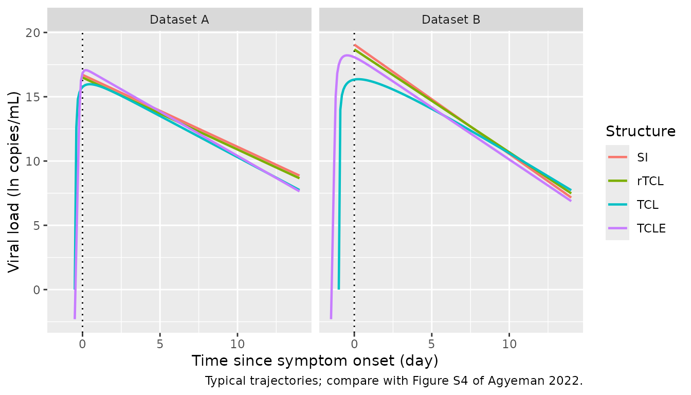
Typical trajectories (Figure S4)
Figure S4 of the Supporting Information shows visual predictive checks on the natural-log scale for each structure and dataset. The plot below shows the typical (population-prediction) trajectory of each packaged model on the same scale; with dataset A the observed medians in Figure S4 sit near 14 ln copies/mL over the first 4 days after symptom onset and fall to about 7 by day 13, and with dataset B they start near 19 and fall to about 9 by day 11. Negative times are the pre-symptomatic phase of the TCL and TCLE models.
ggplot(sim, aes(tsymptom, ln_viral_load, colour = structure)) +
  geom_vline(xintercept = 0, linetype = "dotted") +
  geom_line(linewidth = 0.8) +
  facet_wrap(~dataset) +
  labs(
    x = "Time since symptom onset (day)",
    y = "Viral load (ln copies/mL)",
    colour = "Structure",
    caption = "Typical trajectories; compare with Figure S4 of Agyeman 2022."
  )
Cross-structure agreement
The paper’s main finding is that all four structures describe each dataset similarly and give similar viral decline. The packaged models should therefore agree with each other over the observation window once the initial peak has passed.
agree <- sim |>
  filter(tsymptom >= 5 - 1e-8, tsymptom <= 13 + 1e-8) |>
  mutate(tsymptom = round(tsymptom, 1)) |>
  group_by(dataset, tsymptom) |>
  summarise(
    spread_ln = max(ln_viral_load) - min(ln_viral_load),
    .groups = "drop"
  )
agree |>
  group_by(dataset) |>
  summarise(max_spread_ln = max(spread_ln), .groups = "drop") |>
  dplyr::rename("Dataset" = dataset, "Max spread, days 5-13 (ln copies/mL)" = max_spread_ln) |>
knitr::kable(digits = 2)| Dataset | Max spread, days 5-13 (ln copies/mL) |
|---|---|
| Dataset A | 1.09 |
| Dataset B | 0.76 |
# A transcription error in beta, rho or c (an exponent slip) shifts the
# affected model's trajectory by several ln units; between the faithfully
# transcribed structures the spread is about 1.1 ln units (dataset A) and
# 0.8 (dataset B). The model is deterministic, so this does not vary by machine.
stopifnot(max(agree$spread_ln) < 3)
SI model against its closed form
The SI model has the closed-form solution
V(t) = V(0) * exp(-delta * t). The solver must reproduce
it.
si_ui <- uis[["Agyeman_2022_covid19_si_gastine"]]
si_out <- as.data.frame(rxode2::rxSolve(
  si_ui, rxode2::et(seq(0, 14, by = 0.5)),
  rtol = 1e-10, atol = 1e-12, returnType = "data.frame"
))
#> ℹ omega/sigma items treated as zero: 'etalrbase', 'etaldelta'
closed <- (si_ui$theta[["lrbase"]] - exp(si_ui$theta[["ldelta"]]) * si_out$time) / log(10)
# Measured ~1e-9 under LSODA at these tolerances.
stopifnot(max(abs(si_out$log10_viral_load - closed)) < 1e-6)
NCA
The models describe untreated natural-history viral load with no dosing, so there is no exposure for PKNCA to summarise and the paper reports no NCA metrics. Validation relies on the closed-form R0 / L reproduction and the trajectory checks above.
Sensitivity analysis with rho fixed
Because the TCLE fits gave implausibly large R0 values, the authors refitted TCLE with rho fixed to 10 copies/mL/day (values marked with an asterisk in Tables S2 and S3). These refits are a sensitivity analysis and are not packaged as separate models. Recomputing R0 and L from the printed refit parameters shows that the dataset A row is internally consistent but the dataset B row is not:
rho_fix <- tibble::tribble(
  ~dataset, ~beta, ~delta, ~c, ~R0_paper, ~L_paper,
  "A", 2.28e-4, 0.43, 1.4, 22.21, 2.33,
  "B", 2.08e-4, 0.34, 2.73, 24.09, 2.44
) |>
  mutate(
    R0_recomputed = 10 * beta * 1.3e5 / (delta * (c + beta * 1.3e5)),
    L_recomputed = 1 / delta
  )
rho_fix |>
  mutate(beta = formatC(beta, format = "e", digits = 2)) |>
  dplyr::rename(
    "Dataset" = dataset, "beta" = beta, "delta (1/day)" = delta,
    "c (1/day)" = c, "R0 (paper)" = R0_paper, "L (paper, day)" = L_paper,
    "R0 (recomputed)" = R0_recomputed, "L (recomputed, day)" = L_recomputed
  ) |>
knitr::kable(digits = 3)| Dataset | beta | delta (1/day) | c (1/day) | R0 (paper) | L (paper, day) | R0 (recomputed) | L (recomputed, day) |
|---|---|---|---|---|---|---|---|
| A | 2.28e-04 | 0.43 | 1.40 | 22.21 | 2.33 | 22.207 | 2.326 |
| B | 2.08e-04 | 0.34 | 2.73 | 24.09 | 2.44 | 26.715 | 2.941 |
For dataset B the printed L of 2.44 days implies delta = 0.41/day
rather than the printed 0.34/day, and neither value reproduces the
printed R0 of 24.09, so at least one entry of that column is misprinted.
To use a refit anyway, override the ini() values of the
TCLE model (and lrho <- fixed(log(10))); the incubation
period used for the refits is not reported.
Assumptions and deviations
-
IIV and residual error not reported. Section 2.3
states that log-normal random effects were estimated on every estimated
parameter (with a full covariance matrix where the fit converged,
otherwise diagonal) and that the residual error was additive on the
log-transformed viral load. Neither the variances nor the residual SD
are reported in the paper or its Supporting Information. The etas and
addSdare therefore carried asfixed(0), and the models produce typical-value trajectories only. Stochastic VPCs such as Figure S4 cannot be reproduced. -
Observation scale. The paper fitted the natural log
of viral load (Figures S3 and S4 are in ln copies/mL). The packaged
models observe the library’s canonical
log10_viral_load;ln = log10 * log(10), and an additive SD on the ln scale divides bylog(10)on the log10 scale. -
Sign of the infection term. As printed, Equations 3
and 4 write
dI/dt = -beta*T*V - delta*IanddI1/dt = -beta*T*V - k*I1, which would make the infected-cell populations negative. Figure 1 shows the infection flux moving cells from T into I (or I1), and the tabulated R0 values are reproduced by Equations 6 and 7 only for the standard target-cell-limited model with+beta*T*V. The models use the positive sign. - Time origin. SI and rTCL start at symptom onset with the estimated viral load at onset V(0) and f(0) = 1. TCL and TCLE start at infection with the initial conditions in the Table S2/S3 footnote; symptom onset follows after the incubation period selected by the BIC sensitivity analysis (0.5 day for both models with dataset A; 1 day for TCL and 1.5 days for TCLE with dataset B). The VPCs in Figure S4 confirm that TCL and TCLE were plotted on time since infection.
-
rTCL target-cell state. The rTCL model tracks the
fraction f of target cells remaining. It is stored in the
targetcompartment with initial value 1, sotargetholds a fraction in the rTCL models and a cell density in the TCL and TCLE models. - Censoring. Viral loads below the limit of detection were handled as censored observations in the fit (Section 2.3). Censoring is a property of the data, not of the model, and is not represented in the model files.
- Treatment in dataset B. Dataset B patients received routine treatment, including antivirals, which the authors did not model. The dataset B models describe the viral load as observed under that care.
- rho-fixed refits of TCLE are documented above but not packaged, because the paper presents them as a sensitivity analysis of R0 plausibility rather than as final models.