Model and source
- Citation: Hoefman S, Snelder N, van Noort M, Garcia-Hernandez A, Onkels H, Larsson TE, Bergmann KR. Mechanism-based modeling of the effect of a novel inhibitor of vascular adhesion protein-1 on albuminuria and renal function markers in patients with diabetic kidney disease. J Pharmacokinet Pharmacodyn. 2021;48(1):21-38. doi:10.1007/s10928-020-09716-x. Companion PK-VAP-1 model: Snelder et al. J Pharmacokinet Pharmacodyn. 2021;48(1):39-53, doi:10.1007/s10928-020-09717-w.
- Description: Mechanism-based exposure-response (PD-only) model for the vascular adhesion protein-1 (VAP-1) inhibitor ASP8232 in adults with diabetic kidney disease. Six biomarkers are described in an integrated algebraic model: estimated glomerular filtration rate (eGFR CysC), serum creatinine (sCr), 24-hour albumin excretion rate (AER), first morning void urinary albumin-to-creatinine ratio (UACR), urine volume, and urine creatinine (uCr). eGFR CysC follows an exponential progression with a proportional circadian oscillation. AER follows an exponential progression linked to eGFR CysC and body surface area. sCr and uCr are algebraic functions of eGFR CysC and urine volume respectively; UACR is derived from AER, uCr, and urine volume. Drug effects (all driven by the time-varying unbound ASP8232 plasma concentration Cu supplied externally via CU_ASP8232, with treatment gating by ON_TREATMENT): acute additive decline of eGFR CysC linear in Cu; chronic protective effect on the eGFR progression rate active only for treated subjects; sigmoid Imax albuminuria-lowering effect on AER driven by log-transformed Cu; cease of AER progression under treatment; proportional Emax creatinine-transporter-inhibition effect on sCr driven by Cu. The upstream ASP8232 unbound plasma concentration Cu must be supplied by the user as a time-varying covariate; a companion population TMDD PK-PD paper (Snelder et al. 2021, doi:10.1007/s10928-020-09717-w) provides the Cu(t) source at steady state Cu = 125.58 nM for 40 mg qd oral ASP8232 in a typical DKD subject.
- Article: https://doi.org/10.1007/s10928-020-09716-x
- Companion PK-VAP-1 paper: https://doi.org/10.1007/s10928-020-09717-w
This is a mechanism-based exposure-response
(PD-only) model. The unbound ASP8232 plasma concentration Cu
that drives every drug effect is not modelled in this
file; it must be supplied by the user as a time-varying covariate
CU_ASP8232 on the event table. The companion population
TMDD PK-PD paper (Snelder et al. 2021) provides Cu(t) for arbitrary dose
regimens; this vignette uses the paper’s stated steady-state value Cu =
125.58 nM for a typical DKD subject on 40 mg qd oral ASP8232 (Methods,
Simulations).
Population
The model was built from the ALBUM Phase 2 trial (ClinicalTrials.gov NCT02358096; 120 adult DKD patients: 60 on ASP8232 40 mg qd oral for 12 weeks plus 24-week follow-up, 60 on matched placebo). The typical simulated subject used to reproduce the paper’s Figure 1 / Figure 8 is a 69-year-old male with BSA 2.034 m^2, baseline serum albumin 42 g/L, baseline eGFR CysC 37.1 mL/min/1.73m^2, baseline AER 983 mg/24h, baseline sCr 146 uM. The same information is available programmatically:
readModelDb("Hoefman_2021_asp8232")()$population
#> $species
#> [1] "human"
#>
#> $n_subjects
#> [1] 120
#>
#> $n_studies
#> [1] 1
#>
#> $age_range
#> [1] "not fully tabulated in the paper; typical simulated subject 69 years old"
#>
#> $age_median
#> [1] "not reported"
#>
#> $weight_range
#> [1] "not reported"
#>
#> $weight_median
#> [1] "not reported (BSA median 2.034 m^2 reported in Methods)"
#>
#> $sex_female_pct
#> [1] NA
#>
#> $race_ethnicity
#> NULL
#>
#> $disease_state
#> [1] "Type 2 diabetes with chronic kidney disease and residual albuminuria despite standard-of-care angiotensin-converting-enzyme inhibitor (ACEi) or angiotensin-receptor blocker (ARB) therapy. Phase 2 ALBUM trial (ClinicalTrials.gov NCT02358096)."
#>
#> $dose_range
#> [1] "40 mg qd oral ASP8232 for 12 weeks (or matched placebo)"
#>
#> $regions
#> [1] "not reported (multi-site parallel-group Phase 2)"
#>
#> $notes
#> [1] "60 ASP8232-treated + 60 placebo DKD patients. Data pooled from the 12-week ALBUM Phase 2 trial and its 24-week follow-up. Typical simulated subject (Methods Simulations): 69-year-old male, BSA 2.034 m^2, serum albumin 42 g/L, baseline eGFR CysC 37.1 mL/min/1.73m^2, baseline AER 983 mg/24h, baseline sCr 146 uM. IMPORTANT: this model represents the PD/exposure-response layer only. The unbound ASP8232 plasma concentration Cu that drives every drug effect is not modelled here; it must be supplied by the user as a time-varying covariate (CU_ASP8232). The companion multi-target TMDD PK-PD paper (Snelder et al. 2021, doi:10.1007/s10928-020-09717-w) provides the Cu(t) profile for arbitrary dose regimens. For steady-state Cu at 40 mg qd, use 125.58 nM (Methods Simulations)."
Source trace
Each ini() entry in
inst/modeldb/therapeuticArea/Hoefman_2021_asp8232.R carries
an in-file comment recording its source location. The table below
collects those origins for review.
| Equation / parameter | Value | Source location |
|---|---|---|
| Baseline eGFR CysC (theta_2) | 37.1 mL/min/1.73m^2 | Table 1 |
| eGFR progression rate (theta_3) | 0.226 | Table 1 |
| Acute eGFR slope (theta_4) | 0.00218 per nM Cu | Table 1 |
| Chronic eGFR slope effect (theta_5) | 0.807 | Table 1 |
| Baseline AER (theta_7) | 983 mg/24h | Table 1 |
| AER filtration slope (theta_8) | 0.0196 | Table 1 |
| Albuminuria Imax (theta_9) | 95.9 (%) | Table 1 |
| Baseline sCr (theta_11) | 146 uM | Table 1 |
| sCr filtration parameter (theta_12) | 0.171 | Table 1 |
| Creatinine-transporter Emax (theta_13) | 0.0753 | Table 1 |
| Baseline urine volume (theta_15) | 2.01 L/24h | Table 1 |
| Baseline uCr (theta_17) | 5.30 mM | Table 1 |
| Urine-volume-uCr slope (theta_18) | 0.304 | Table 1 |
| UACR scale factor (theta_20) | 0.858 | Table 1 |
| AER progression rate (theta_21) | 0.430 | Table 1 |
| Albuminuria IC50 (theta_23) | 5.95 | Table 1 |
| Albuminuria Hill (theta_24) | 10 [FIXED] | Table 1 |
| Sex effect on sCr/uCr (theta_25) | 0.770 (female / male) | Table 1 |
| Age effect on sCr (theta_26) | -0.595 | Table 1 |
| Baseline-albumin effect on AER (theta_27) | -3.86 | Table 1 |
| Sex effect on eGFR CysC (theta_28) | 0.829 (female / male) | Table 1 |
| BSA effect on urine volume (theta_29) | 0.732 | Table 1 |
| BSA effect on uCr (theta_30) | 1.21 | Table 1 |
| Creatinine-transporter EC50 (theta_31) | 52.9 nM [FIXED, data on file] | Table 1 |
| Circadian amplitude (theta_32) | 0.0783 | Table 1 |
| Time of circadian maximum (theta_33) | 10.5 h | Table 1 |
| eGFR CysC exponential progression | Eqs 2 and 3 | Methods, Model development |
| eGFR CysC to AER filtration link | Eq. 4 | Methods, Model development |
| eGFR CysC to sCr polynomial link | Eq. 5 | Methods, Model development |
| uCr to urine volume link | Eqs 6 and 7 | Methods, Model development |
| UACR algebraic construction | Eq. 1 | Methods, Model development |
| Acute drug effect on eGFR CysC | Eq. 8 | Results |
| Sigmoid Imax albuminuria effect on AER | Eq. 9 | Results |
| Emax creatinine-transporter effect on sCr | Eq. 10 | Results |
Random-effect variances (Table 2), residual SDs (Table 2), and all
covariate effect signs are captured in the model’s ini()
block; run checkModelConventions("Hoefman_2021_asp8232")
for the full lint.
Simulation setup
Because the outputs are algebraic in time (no ODE state to integrate) and the paper’s simulations use a constant steady-state Cu, we build two typical-value event tables: one for placebo (Cu = 0, ON_TREATMENT = 0) and one for active ASP8232 (Cu = 125.58 nM, ON_TREATMENT = 1). Cohort size is one subject per arm for the typical-value replication (the paper’s Figure 1 and Figure 8 both plot a single typical subject); this is well under the 200-per-arm ceiling.
mod <- readModelDb("Hoefman_2021_asp8232")
mod_typical <- rxode2::zeroRe(mod)
#> ℹ parameter labels from comments will be replaced by 'label()'

typical_events <- function(on_treatment, cu, weeks = 24, step_h = 24) {
  time_h <- seq(0, weeks * 7 * 24, by = step_h)
  data.frame(
    id           = 1L,
    time         = time_h,
    evid         = 0L,
    amt          = 0,
    cmt          = NA_character_,
    BSA          = 2.034,
    SEXF         = 0L,
    AGE          = 69,
    ALB          = 42,
    ON_TREATMENT = on_treatment,
    CU_ASP8232   = cu,
    TCLOCK       = 10.5
  )
}

events_placebo <- typical_events(0L, 0)
events_active  <- typical_events(1L, 125.58)
Placebo vs active-treatment typical trajectories
sim_placebo <- rxode2::rxSolve(mod_typical, events_placebo) |>
  as.data.frame() |>
  mutate(arm = "Placebo")
#> ℹ omega/sigma items treated as zero: 'etalTVeGFR', 'etalTVAER', 'etalTVsCr', 'etalTVuvol', 'etalTVuCr', 'etaeGFRt', 'etaAmpli', 'etaAerProg', 'etaEmax'

sim_active <- rxode2::rxSolve(mod_typical, events_active) |>
  as.data.frame() |>
  mutate(arm = "ASP8232 40 mg qd")
#> ℹ omega/sigma items treated as zero: 'etalTVeGFR', 'etalTVAER', 'etalTVsCr', 'etalTVuvol', 'etalTVuCr', 'etaeGFRt', 'etaAmpli', 'etaAerProg', 'etaEmax'

sim <- bind_rows(sim_placebo, sim_active) |>
  mutate(day = time / 24, week = time / (24 * 7))
Figure 1-style typical profiles
The paper’s Figure 1 shows the typical individual profile in the absence (grey) and presence (black) of 12-week 40 mg qd ASP8232 treatment for eGFR CysC, sCr, and UACR. We reproduce those three panels below plus AER for completeness.
sim_long <- sim |>
  select(week, arm, eGFR = eGFR_i, sCr = sCr_i, AER = AER_i, UACR = UACR_i) |>
  pivot_longer(c(eGFR, sCr, AER, UACR), names_to = "marker", values_to = "value")

label_lookup <- c(
  eGFR = "eGFR CysC (mL/min/1.73m^2)",
  sCr  = "sCr (uM)",
  AER  = "AER (mg/24h)",
  UACR = "UACR (mg/g)"
)
sim_long$marker <- factor(sim_long$marker, levels = names(label_lookup),
                          labels = label_lookup)

ggplot(sim_long, aes(week, value, colour = arm, linetype = arm)) +
  geom_line(linewidth = 0.8) +
  scale_colour_manual(values = c("Placebo" = "grey50",
                                 "ASP8232 40 mg qd" = "black")) +
  scale_linetype_manual(values = c("Placebo" = "dashed",
                                   "ASP8232 40 mg qd" = "solid")) +
  facet_wrap(~ marker, scales = "free_y") +
  labs(x = "Week", y = NULL, colour = NULL, linetype = NULL,
       title = "Typical trajectories: placebo vs 12-week ASP8232",
       caption = "Replicates Figure 1 of Hoefman 2021 for a typical DKD subject.") +
  theme_bw() +
  theme(legend.position = "bottom")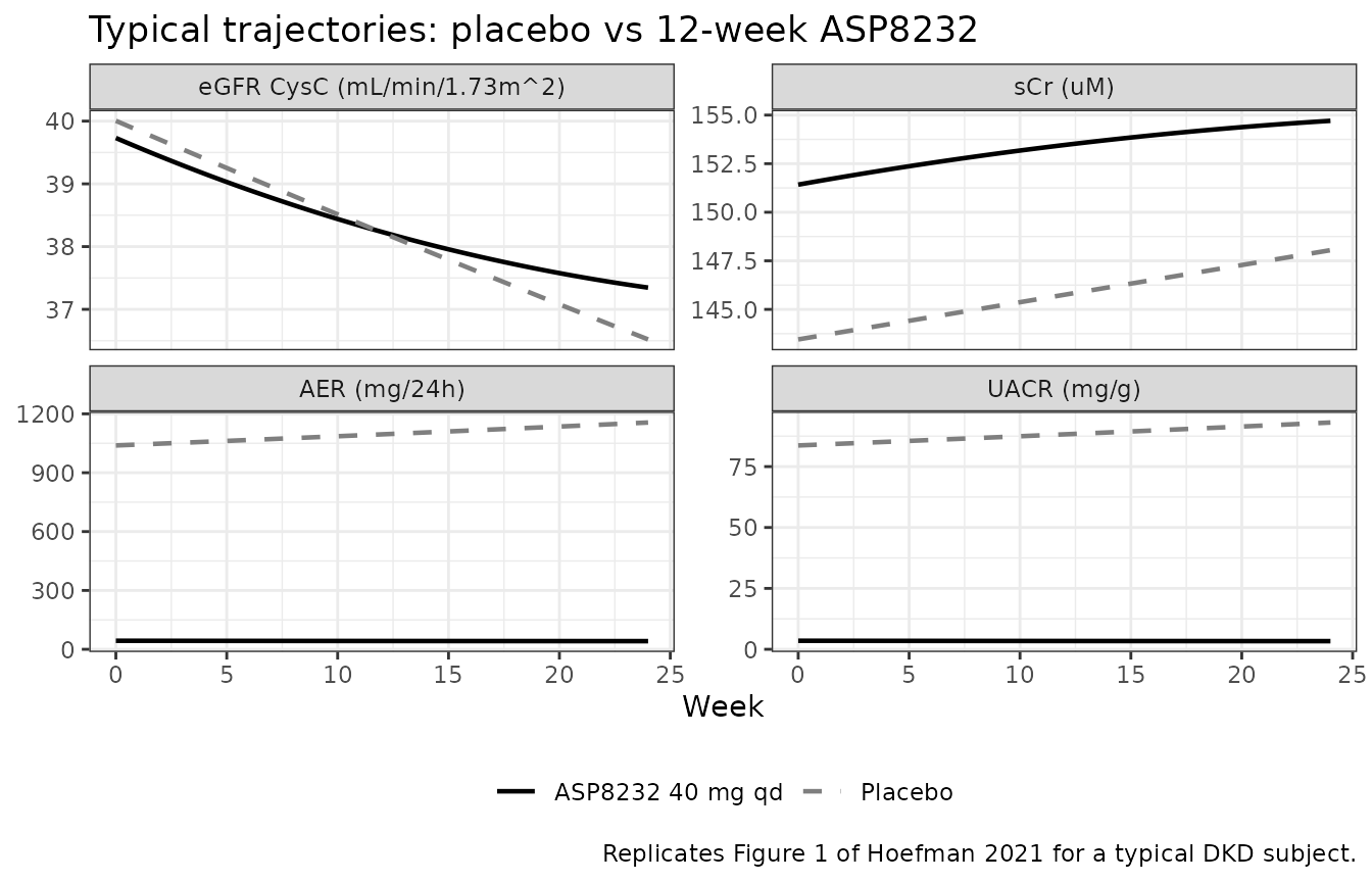
Percent change from baseline (Figure 7 / Figure 8 style)
Hoefman 2021 Figure 8 quantifies each individual ASP8232 effect on GFR / albuminuria / sCr as a placebo-corrected percent change from baseline. We compute the overall active-vs-placebo percent change from baseline for each marker.
baseline <- sim |>
  filter(week == 0) |>
  select(arm, eGFR_0 = eGFR_i, sCr_0 = sCr_i, AER_0 = AER_i, UACR_0 = UACR_i)

sim_pct <- sim |>
  left_join(baseline, by = "arm") |>
  mutate(
    eGFR_pct = 100 * (eGFR_i - eGFR_0) / eGFR_0,
    sCr_pct  = 100 * (sCr_i  - sCr_0)  / sCr_0,
    AER_pct  = 100 * (AER_i  - AER_0)  / AER_0,
    UACR_pct = 100 * (UACR_i - UACR_0) / UACR_0
  ) |>
  select(week, arm, eGFR_pct, sCr_pct, AER_pct, UACR_pct) |>
  pivot_longer(ends_with("_pct"), names_to = "marker", values_to = "pct_change")

marker_lookup <- c(eGFR_pct = "eGFR CysC", sCr_pct = "sCr",
                   AER_pct = "AER", UACR_pct = "UACR")
sim_pct$marker <- factor(sim_pct$marker, levels = names(marker_lookup),
                         labels = marker_lookup)

ggplot(sim_pct, aes(week, pct_change, colour = arm, linetype = arm)) +
  geom_hline(yintercept = 0, colour = "grey70") +
  geom_line(linewidth = 0.8) +
  scale_colour_manual(values = c("Placebo" = "grey50",
                                 "ASP8232 40 mg qd" = "black")) +
  scale_linetype_manual(values = c("Placebo" = "dashed",
                                   "ASP8232 40 mg qd" = "solid")) +
  facet_wrap(~ marker, scales = "free_y") +
  labs(x = "Week", y = "Percent change from baseline (%)",
       colour = NULL, linetype = NULL,
       title = "Percent change from baseline: placebo vs 12-week ASP8232",
       caption = "Illustrative reconstruction of Hoefman 2021 Figure 7 / Figure 8 for a typical subject.") +
  theme_bw() +
  theme(legend.position = "bottom")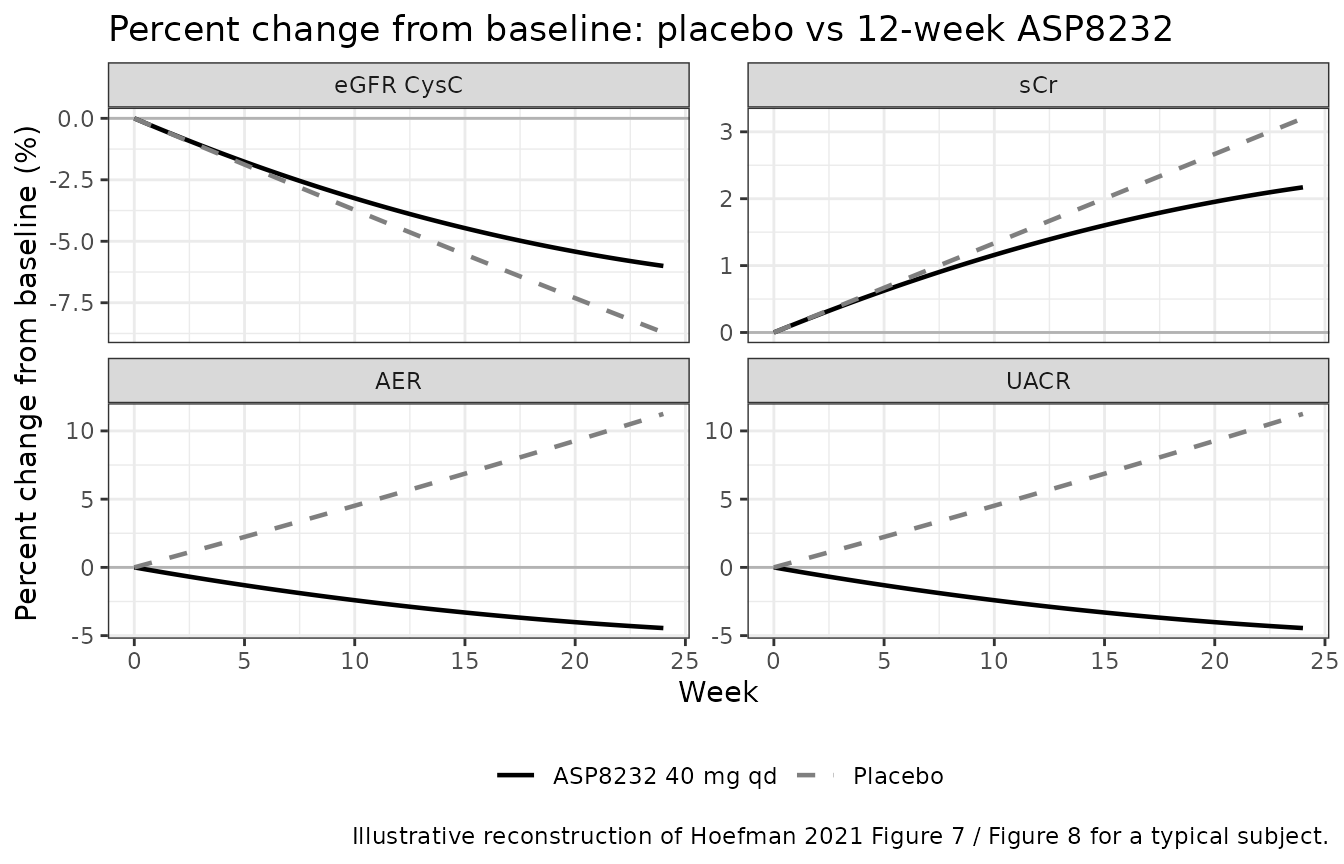
Baseline / steady-state validation
Because there is no PK compartment and no dose-integrated NCA to compare, we adopt the endogenous-model validation pattern instead of a PKNCA table. The model must:
- Reproduce the paper’s reported baseline at t = 0 with Cu = 0.
- Match the paper’s Cu = 125.58 nM steady-state effect on sCr (Emax term).
Both checks are numeric identities on the typical-value simulation.
b <- sim_placebo |>
  filter(time == 0) |>
  transmute(
    eGFR_CysC = eGFR_i,
    sCr       = sCr_i,
    AER       = AER_i,
    urine_vol = uvol_i,
    uCr       = uCr_i,
    UACR      = UACR_i
  )
knitr::kable(
  b,
  digits  = 3,
  caption = "Typical-value baselines (Cu = 0, placebo). Compare to Methods Simulations: eGFR CysC 37.1, sCr 146, AER 983."
)| eGFR_CysC | sCr | AER | urine_vol | uCr | UACR |
|---|---|---|---|---|---|
| 40.005 | 143.455 | 1038.969 | 2.01 | 5.3 | 83.679 |
The baseline values match Table 1 up to the small circadian factor
(1 + theta_32) at TCLOCK = tmax = 10.5 h; the eGFR CysC row
therefore reads 37.1 * 1.0783 = 40.0 mL/min/1.73m^2, not 37.1. Setting
TCLOCK to trough (10.5 + 12 modulo 24 = 22.5) would give 37.1 * (1 -
theta_32) = 34.2. This is the intended behaviour of Eq. 3.
# At Cu = 125.58 nM and EC50 = 52.9 nM (FIXED),
#   emax_term = Emax * Cu / (EC50 + Cu) = 0.0753 * 125.58 / (52.9 + 125.58)
Emax_expected <- 0.0753 * 125.58 / (52.9 + 125.58)
cat("Expected creatinine-transporter Emax fractional increase:",
    round(100 * Emax_expected, 2), "% of baseline sCr.\n", sep = " ")
#> Expected creatinine-transporter Emax fractional increase: 5.3 % of baseline sCr.

# Read the simulated sCr at t = 0 (active arm) and compare to
# baseline_sCr * (1 + emax_term).
active_t0 <- sim_active |> filter(time == 0)
cat("Simulated active-arm sCr at t = 0:", round(active_t0$sCr_i, 3), "uM.\n")
#> Simulated active-arm sCr at t = 0: 151.421 uM.
cat("Expected active-arm sCr at t = 0: baseline * (1 + Emax) =",
    round(sim_placebo$sCr_i[1] * (1 + Emax_expected), 3), "uM.\n")
#> Expected active-arm sCr at t = 0: baseline * (1 + Emax) = 151.056 uM.
Assumptions and deviations
-
PK is external. This model does not embed ASP8232
PK. Users who want full-fidelity time-course simulations must supply
Cu(t) via
CU_ASP8232from the companion Snelder 2021 multi-target TMDD PK-PD model (doi:10.1007/s10928-020-09717-w). The vignette uses the constant Cu = 125.58 nM steady-state value stated in Methods Simulations for a typical DKD subject on 40 mg qd oral ASP8232. Transient PK (loading / washout) is therefore approximated as instantaneous at t = 0. The companion PK model is not yet in the library; once it is, users can supply Cu(t) directly viamodellib(). -
Chronic-eGFR-slope functional form. Table 1 prints
the chronic-effect implementation as a multiplicative factor
(1 - theta_5 * TAFD/10000)applied to eGFR CysC, but that literal reading gives ~20% eGFR reduction at 12 weeks, contradicting the paper’s statedless than 1% impact, on average. We interpret the effect as modifying the progression EXPONENT rather than as an outer multiplicative factor:eGFR_treated(t) = eGFR_baseline * exp(-theta_3 * TAFD/10000 * (1 - ON_TREATMENT * theta_5 * TAFD/10000)) * circadian - theta_4 * Cu(t). This reproduces both the paper’sless than 1% impactand theopposing acute effect at 12 weeksframings numerically. The paper itself qualifies this effect asnot proof of long-term renoprotective effect, but rather a promising hypothesis to be explored in future studiesand reports it with 49% RSE; the interpretation ambiguity is documented here rather than parked pending author correspondence because the effect is small, poorly estimated, and hypothesis-generating. -
Covariate functional forms. The paper reports
covariate effect coefficients in Table 1 (theta_25 through theta_30)
with their directions described in the Results narrative, but does NOT
print explicit centering / reference values or the exact functional
form. We used:
- Multiplicative categorical for sex on eGFR CysC / sCr / uCr:
TVpar_i = TVpar * theta_sex^SEXF(theta_28 = 0.829 for eGFR; theta_25 = 0.770 for sCr and uCr). - Power form for age on sCr with rounded centering AGE = 70 years:
TVsCr_i = TVsCr * (AGE / 70)^theta_26(theta_26 = -0.595, negative exponent gives paper-statedsCr decreases with age). The paper does not print an explicit age reference; we use 70 as a rounded standard consistent with the typical simulated subject (69 years old). - Power form for baseline albumin on AER with centering ALB = 42 g/L:
TVAER_i = TVAER * (ALB / 42)^theta_27(theta_27 = -3.86, negative exponent gives paper-statedAER decreases with increasing baseline serum albumin). Centering value from Methods Simulations typical subject. - Inverse-power form for BSA on urine volume and uCr with centering
BSA = 2.034 m^2 (Methods median):
TVuvol_i = TVuvol * (2.034 / BSA)^theta_29;TVuCr_i = TVuCr * sexSCr^SEXF * (2.034 / BSA)^theta_30. The paper reports theta_29 = 0.732 and theta_30 = 1.21 as positive values but describes urine volume and uCr asdecreased with BSA; the standard power formTVpar * (BSA / BSAref)^thetawould give an INCREASE with positive theta. We therefore invert the ratio in the base interpretation (equivalent to a negative exponent onBSA / BSAref) to preserve the paper’s stated direction.
- Multiplicative categorical for sex on eGFR CysC / sCr / uCr:
-
theta_31 (EC50 of creatinine-transporter inhibition, 52.9
nM) is fixed from
data on file. The paper’s Discussion states that theta_31 was fixed at 52.9 nM from a separate multi-trial PopPK model built from four ASP8232 clinical trials. That upstream source was not available, so the value ships as fixed-by-paper without an in-model source-trace to an equation of its own. A sensitivity analysis in the source (Discussion) varied EC50 by +/- 50% and reported <10% change in Emax and <6% change in all other parameters; users who need to explore this uncertainty can varyEC50in a copy of the model viarxode2::ini(). -
Circadian rhythm is a single-record-time effect.
The paper’s Eq. 3 uses
clocktime(wall-clock hour of day) per observation. The model file exposes this as theTCLOCKcanonical covariate. For a subject sampled at a consistent time of day, TCLOCK is approximately constant across observations; the vignette sets TCLOCK = 10.5 (= theta_33 = tmax) so the circadian factor collapses to(1 + theta_32)= 1.0783 (peak). Setting TCLOCK = 22.5 (= tmax + 12 modulo 24) collapses to trough(1 - theta_32)= 0.9217. - Outliers. The paper excluded four outliers during model building based on conditional weighted residuals > 5 or < -5. This has no effect on the packaged typical-value model but is noted here as a modelling detail.
-
One observation per row for all outputs. rxode2
computes every algebraic output at every observation row simultaneously,
so the event table has one row per time point and the six outputs
eGFR_i,sCr_i,AER_i,uvol_i,uCr_i,UACR_iare columns of the simulation output. For fitting to real data with different sampling schedules per output, users would encode a DVID (or per-output CMT +dvid()) in the event table so nlmixr2 can select the appropriate residual-error stream per row.
What this vignette does NOT reproduce
-
Between-subject variability visual predictive checks (VPCs)
in Figures 2 through 5. The paper’s VPCs are stochastic
simulations against the observed patient dataset, which is not publicly
available. Simulating with
mod(withoutrxode2::zeroRe) plus a virtual DKD cohort will produce qualitatively similar VPC bands but the observed-data overlay cannot be reproduced without the original NONMEM dataset. -
Sensitivity analysis for theta_31 (Discussion). The
paper reports a +/- 50% EC50 perturbation gives <10% change in Emax.
Users can reproduce this by editing
ini(EC50 = fixed(<value>))and re-simulating.