Bietti crystalline dystrophy BCVA natural history (Zhang 2025)
Source:vignettes/articles/Zhang_2025_bietti_crystalline_dystrophy_mbma.Rmd
Zhang_2025_bietti_crystalline_dystrophy_mbma.RmdModel and source
- Citation: Zhang H, Yin S, Guan N, Wang J, Cheng Q, Zhang L, Zheng Q, Lv H, Wei W. Natural history of progressive vision loss in Bietti crystalline dystrophy: a model-based meta-analysis. BMJ Open Ophthalmology 2025;10:e001908. doi:10.1136/bmjophth-2024-001908.
- Article: https://doi.org/10.1136/bmjophth-2024-001908
- Supplement (data analysis protocols, appendices 1-12): published online only with the article; the parameter table used below is supplement appendix 7.
Bietti crystalline corneoretinal dystrophy (BCD) is an autosomal-recessive retinal degeneration caused by biallelic mutations in CYP4V2. There is no approved treatment, and CYP4V2 gene-therapy programmes need a quantitative description of the untreated trajectory of vision loss in order to size and interpret their trials. Zhang 2025 supplies that description as a model-based meta-analysis: individual eye-level best-corrected visual acuity (BCVA) time courses were reconstructed from 14 published studies and fitted with a single linear disease-progression model.
The structural model (supplement equation 1, where the supplement writes the slope as ) is
with an exponential between-individual random effect on the slope (supplement equation 2) and additive residual error on the LogMAR scale (supplement equation 4):
Four features are worth flagging before any simulation:
- LogMAR is inverted relative to intuition. LogMAR is the base-10 logarithm of the minimum angle of resolution, so higher LogMAR means worse vision. A positive slope therefore encodes progressive vision loss. Zhang 2025 phrases every result as “BCVA increased by … LogMAR per year”, meaning acuity deteriorated.
- No intercept. The model has exactly one structural parameter. Time zero is the first visual-acuity evaluation, so the predicted change from baseline is identically zero at by construction.
- The random effect is between-EYE, not between-study. This is unusual for a meta-analysis. Because individual participant data were reconstructed from each source publication rather than pooled as study-level summaries, Zhang 2025 estimated an individual-level and reported no study-level variance term. The packaged model consequently simulates eye-level trajectories and cannot separate between-study from between-eye heterogeneity (see Assumptions and deviations).
-
Every covariate was screened out. Age, age at
onset, disease duration, baseline BCVA, sex, race, CYP4V2
genotype and family history were all tested and none was retained, so
the base model is the final model (supplement appendix 6). They
are recorded in the model file’s
covariatesDataExcludedmetadata and inpopulation$notesrather than incovariateData.
mod  <- readModelDb("Zhang_2025_bietti_crystalline_dystrophy_mbma")
ui   <- rxode2::rxode(mod)
mod0 <- rxode2::zeroRe(mod)   # typical-value model: no IIV, no residual error
Population
- 14 published studies, 117 patients, 193 study eyes (84 left, 109 right). All eyes untreated – prior treatment was an exclusion criterion, and there is no approved therapy for BCD.
- Age at first BCVA recording: median 49.0 years (range 15.0-76.0) (supplement appendix 2).
- Age at onset: median 47.0 years (range 11.0-76.0). Where onset age was not reported the age at first BCVA recording was substituted.
- Disease duration: median 8.00 years (range 0.500-47.0), defined as age minus age of onset plus the longest visit.
- Baseline BCVA: median 0.150 LogMAR (range -0.200 to 2.60). 151 of the 193 eyes had baseline BCVA below 0.5 LogMAR and 42 at or above it.
- Sex: 77 of 117 patients female (65.8%).
- Race: 80 of 117 patients East Asian (68.4%), 37 non-East Asian (31.6%). Six studies enrolled East Asian and nine non-East Asian populations; one study contributed to both strata, which is why the study counts sum to 15 rather than 14.
-
CYP4V2 genotype: c.802-8_810de117insGC
(exon 7 deletion) homozygous or compound heterozygous in 53 patients,
other genotypes in 36, not determined in
- Family history of BCD: 11 of 117 patients (9.4%).
Off-chart acuities were coded on the LogMAR scale as 1.9 (counting fingers), 2.3 (hand motion), 2.7 (light perception) and 3.0 (no light perception), so 3.0 LogMAR is the ceiling of the measurement scale – total blindness.
The same information is available programmatically:
str(ui$population, max.level = 1)
#> List of 19
#>  $ species                : chr "human"
#>  $ n_subjects             : int 117
#>  $ n_eyes                 : int 193
#>  $ n_studies              : int 14
#>  $ age_range              : chr "15.0-76.0 years (Zhang 2025 supplement appendix 2, age at the first BCVA recording)"
#>  $ age_median             : chr "49.0 years (Zhang 2025 supplement appendix 2)"
#>  $ weight_range           : chr NA
#>  $ weight_median          : chr NA
#>  $ sex_female_pct         : num 65.8
#>  $ race_ethnicity         : Named num [1:2] 68.4 31.6
#>   ..- attr(*, "names")= chr [1:2] "East Asian" "Non-East Asian"
#>  $ disease_state          : chr "Bietti crystalline corneoretinal dystrophy (BCD), an autosomal-recessive progressive retinal degeneration cause"| __truncated__
#>  $ dose_range             : chr "n/a (untreated natural history; the model has no drug input)"
#>  $ regions                : chr "Six of the 14 included studies enrolled East Asian populations (China, Japan, Korea) and nine enrolled non-East"| __truncated__
#>  $ onset_age_range        : chr "11.0-76.0 years (Zhang 2025 supplement appendix 2; where the age of onset was missing the age at the first BCVA"| __truncated__
#>  $ onset_age_median       : chr "47.0 years (Zhang 2025 supplement appendix 2)"
#>  $ disease_duration_range : chr "0.500-47.0 years (Zhang 2025 supplement appendix 2; duration = age - age of onset + longest visit)"
#>  $ disease_duration_median: chr "8.00 years (Zhang 2025 supplement appendix 2)"
#>  $ baseline_bcva          : chr "Median 0.150 LogMAR [-0.200, 2.60] (Zhang 2025 supplement appendix 2). Of the 193 study eyes, 151 had baseline "| __truncated__
#>  $ notes                  : chr "Individual eye-level BCVA time courses were reconstructed from 14 published studies retrieved by a PRISMA-style"| __truncated__
Source trace
| Item | Value | Source location |
|---|---|---|
bcvacfb <- slope * time |
n/a | Supplement, Data analysis, equation (1)
(Effect = K x Time) |
| Exponential between-individual random effect | n/a | Supplement, Data analysis, equation (2); appendix 4
model 102 (ETA: Exponential type), selected as the base
model |
| Additive residual error | n/a | Supplement, Data analysis, equation (4); appendix 4
model 102 (SIGMA: Additive type) |
| No covariate on the slope | n/a | Supplement appendix 6 (forward inclusion + backward elimination; nothing retained) |
lslope = log(0.0566) |
K = 0.0566 LogMAR/year (RSE 10.1%, 95% CI 0.0454-0.0678) | Supplement appendix 7, Final model,
Parameter of population / K
|
etalslope ~ 0.898^2 |
omega(K) = 0.898 (RSE 8.7%, 95% CI 0.745-1.05) | Supplement appendix 7,
Between-individual random effect parameters / omega (K)
|
addSd = 0.336 |
sigma(ADD) = 0.336 (RSE 5.3%, 95% CI 0.301-0.371) | Supplement appendix 7,
Intra-individual random effect parameters / sigma (ADD)
|
| Bootstrap corroboration | K 0.0564 (0.0452-0.0694); omega 0.894 (0.700-1.08); sigma 0.336 (0.205-0.446) | Supplement appendix 7, Bootstrap (1000 successes) columns |
omega and sigma are standard deviations, not variances
The supplement pins the scale of its own random-effect parameters
explicitly. After equations (2) and (3) it states that
“conform[s] to a normal distribution with mean 0 and
variance
”,
and after equations (4) to (6) that
and
“conform to a normal distribution with mean 0 and
variance
and
”.
The reported omega (K) = 0.898 and
sigma (ADD) = 0.336 are therefore standard
deviations. ini() in nlmixr2 takes a
variance for an eta, hence etalslope ~ 0.898^2,
and an SD for add(), hence
addSd <- 0.336 unchanged.
This ambiguity is worth resolving explicitly because it is a common
transcription error, but note that here it is nearly immaterial: reading
0.898 as a variance instead would give an SD of 0.948
rather than 0.898, a difference of only 5.5% in the log-scale SD.
Verification 1: the typical-value trajectory is the published closed form
zeroRe() removes both the between-eye random effect and
the residual error, leaving the deterministic prediction. It must equal
0.0566 * t exactly, and must be exactly zero at time
zero.
t_grid <- seq(0, 8, by = 0.5)
ev_typ <- data.frame(id = 1L, time = t_grid, evid = 0L, amt = 0)

sim_typ <- rxode2::rxSolve(mod0, events = ev_typ, returnType = "data.frame")
#> ℹ omega/sigma items treated as zero: 'etalslope'

# 0.0566 is transcribed from Zhang 2025 supplement appendix 7 -- it is NOT read
# back out of the model, so a mistyped lslope makes this assertion go red.
closed_form <- 0.0566 * t_grid

stopifnot(
  # Deterministic quantities: assert tightly (no cohort, no RNG involved).
  isTRUE(all.equal(sim_typ$bcvacfb, closed_form, tolerance = 1e-10)),
  # No intercept: change from baseline is identically zero at the baseline visit.
  sim_typ$bcvacfb[t_grid == 0] == 0
)

cat("max |model - 0.0566 * t| =",
    format(max(abs(sim_typ$bcvacfb - closed_form)), digits = 3), "LogMAR\n")
#> max |model - 0.0566 * t| = 1.11e-16 LogMAR
Verification 2: reproduce the published simulation tables
Zhang 2025 table 2 and supplement appendix 10 report the simulated
change from baseline in BCVA at half-yearly intervals out to 8 years,
for the whole cohort and for five subgroups. The subgroup slopes are
post-hoc empirical-Bayes summaries of the individual
values, not fitted covariate effects (no covariate survived
screening), so they are reproduced here by overriding
lslope rather than by adding a covariate to the model.
published <- tibble::tribble(
  ~time, ~all,  ~all_lo, ~all_hi, ~sev,  ~bcva_lo_grp, ~bcva_hi_grp, ~onset_lt40, ~onset_ge40,
   0.5,  0.03,  0.02,    0.03,    0.05,  0.04,         0.05,         0.03,        0.04,
   1.0,  0.06,  0.05,    0.07,    0.09,  0.08,         0.10,         0.07,        0.09,
   1.5,  0.09,  0.07,    0.10,    0.14,  0.12,         0.15,         0.10,        0.13,
   2.0,  0.11,  0.09,    0.14,    0.18,  0.15,         0.20,         0.14,        0.18,
   2.5,  0.14,  0.12,    0.17,    0.23,  0.19,         0.25,         0.17,        0.22,
   3.0,  0.17,  0.14,    0.21,    0.27,  0.23,         0.30,         0.20,        0.27,
   3.5,  0.20,  0.16,    0.24,    0.32,  0.27,         0.34,         0.24,        0.31,
   4.0,  0.23,  0.19,    0.27,    0.36,  0.31,         0.39,         0.27,        0.36,
   4.5,  0.26,  0.21,    0.31,    0.41,  0.35,         0.44,         0.31,        0.40,
   5.0,  0.29,  0.23,    0.34,    0.45,  0.39,         0.49,         0.34,        0.45,
   5.5,  0.31,  0.26,    0.38,    0.50,  0.42,         0.54,         0.37,        0.49,
   6.0,  0.34,  0.28,    0.41,    0.54,  0.46,         0.59,         0.41,        0.54,
   6.5,  0.37,  0.30,    0.45,    0.59,  0.50,         0.64,         0.44,        0.58,
   7.0,  0.40,  0.33,    0.48,    0.63,  0.54,         0.69,         0.48,        0.63,
   7.5,  0.43,  0.35,    0.52,    0.68,  0.58,         0.74,         0.51,        0.67,
   8.0,  0.46,  0.37,    0.55,    0.72,  0.62,         0.79,         0.54,        0.72
)
# Columns `all`, `all_lo`, `all_hi` and `sev` are Zhang 2025 table 2 (main text);
# `bcva_lo_grp`, `bcva_hi_grp`, `onset_lt40` and `onset_ge40` are supplement
# appendix 10.

# Slope of a straight line forced through the origin. Because the published
# model has no intercept, this recovers the K that generated each column.
slope_through_origin <- function(t, y) sum(t * y) / sum(t^2)
The published columns are internally consistent with
Effect = K * t
Each published column should be recoverable as K * t for
the K the paper reports for that group. Rounding to two
decimals is the dominant error at short times, so the whole column is
summarised by a single regression through the origin.
groups <- tibble::tribble(
  ~Group,                                                  ~column,       ~`Published K`, ~`K source`, ~n_eyes,
  "All included eyes",                                     "all",          0.0566,        "Supplement appendix 7 (model estimate)", 193L,
  "Baseline BCVA < 0.5 LogMAR",                            "bcva_lo_grp",  0.0766,        "Results, post-hoc Bayesian",             151L,
  "Baseline BCVA >= 0.5 LogMAR",                           "bcva_hi_grp",  0.0979,        "Results, post-hoc Bayesian",              42L,
  "Onset age < 40 years",                                  "onset_lt40",   0.0675,        "Results, post-hoc Bayesian",              71L,
  "Onset age >= 40 years",                                 "onset_ge40",   0.0892,        "Results, post-hoc Bayesian",             122L,
  "BCVA >= 0.5 LogMAR and duration >= 10 years",           "sev",          0.0900,        "Results, post-hoc Bayesian",              15L
) |>
  dplyr::rowwise() |>
  dplyr::mutate(
    `Recovered K` = slope_through_origin(published$time, published[[column]]),
    `Diff (%)`    = 100 * (`Recovered K` - `Published K`) / `Published K`
  ) |>
  dplyr::ungroup()

# Deterministic: both sides are hardcoded transcriptions of the paper. A
# published table that did not come from `Effect = K * t` would fail this.
stopifnot(max(abs(groups$`Diff (%)`)) < 2)

groups |>
  dplyr::select(Group, n_eyes, `Published K`, `Recovered K`, `Diff (%)`, `K source`) |>
  dplyr::rename("Eyes" = n_eyes) |>
  knitr::kable(digits = c(0, 0, 4, 4, 2, 0),
caption = "Regression through the origin of each published simulation column recovers that group's published K.")| Group | Eyes | Published K | Recovered K | Diff (%) | K source |
|---|---|---|---|---|---|
| All included eyes | 193 | 0.0566 | 0.0572 | 1.02 | Supplement appendix 7 (model estimate) |
| Baseline BCVA < 0.5 LogMAR | 151 | 0.0766 | 0.0772 | 0.76 | Results, post-hoc Bayesian |
| Baseline BCVA >= 0.5 LogMAR | 42 | 0.0979 | 0.0985 | 0.57 | Results, post-hoc Bayesian |
| Onset age < 40 years | 71 | 0.0675 | 0.0680 | 0.67 | Results, post-hoc Bayesian |
| Onset age >= 40 years | 122 | 0.0892 | 0.0896 | 0.42 | Results, post-hoc Bayesian |
| BCVA >= 0.5 LogMAR and duration >= 10 years | 15 | 0.0900 | 0.0904 | 0.48 | Results, post-hoc Bayesian |
The packaged model reproduces Zhang 2025 table 2
solve_typical_slope <- function(k) {
  rxode2::rxSolve(
    rxode2::zeroRe(rxode2::ini(mod, lslope = log(k))),
    events     = data.frame(id = 1L, time = published$time, evid = 0L, amt = 0),
    returnType = "data.frame"
  )$bcvacfb
}

table2 <- published |>
  dplyr::transmute(
    time,
    Published    = all,
    Model        = solve_typical_slope(0.0566),
    Difference   = Model - Published
  )
#> ℹ change initial estimate of `lslope` to `-2.871746293773`
#> ℹ omega/sigma items treated as zero: 'etalslope'

# Deterministic. Realised maximum is ~0.007 LogMAR, which is the two-decimal
# rounding of the published column; 0.01 leaves headroom for that rounding and
# still goes red on a third-significant-figure error in K at t = 8 y.
stopifnot(max(abs(table2$Difference)) < 0.01)

table2 |>
  dplyr::rename(
    "Time (years)"                        = time,
    "Published (LogMAR)"                  = Published,
    "Packaged model (LogMAR)"             = Model,
    "Difference (LogMAR)"                 = Difference
  ) |>
  knitr::kable(digits = c(1, 2, 4, 4),
caption = "Zhang 2025 table 2, 'All included population (193 eyes)' column vs the packaged model's typical-value prediction.")| Time (years) | Published (LogMAR) | Packaged model (LogMAR) | Difference (LogMAR) |
|---|---|---|---|
| 0.5 | 0.03 | 0.0283 | -0.0017 |
| 1.0 | 0.06 | 0.0566 | -0.0034 |
| 1.5 | 0.09 | 0.0849 | -0.0051 |
| 2.0 | 0.11 | 0.1132 | 0.0032 |
| 2.5 | 0.14 | 0.1415 | 0.0015 |
| 3.0 | 0.17 | 0.1698 | -0.0002 |
| 3.5 | 0.20 | 0.1981 | -0.0019 |
| 4.0 | 0.23 | 0.2264 | -0.0036 |
| 4.5 | 0.26 | 0.2547 | -0.0053 |
| 5.0 | 0.29 | 0.2830 | -0.0070 |
| 5.5 | 0.31 | 0.3113 | 0.0013 |
| 6.0 | 0.34 | 0.3396 | -0.0004 |
| 6.5 | 0.37 | 0.3679 | -0.0021 |
| 7.0 | 0.40 | 0.3962 | -0.0038 |
| 7.5 | 0.43 | 0.4245 | -0.0055 |
| 8.0 | 0.46 | 0.4528 | -0.0072 |
The published 95% CI is parameter uncertainty, not a prediction interval
Table 2 reports a 95% CI around each simulated value. Those intervals are narrow and scale exactly in proportion to time, which is the signature of uncertainty in the typical rather than of between-eye variability. Regressing the lower and upper CI columns through the origin should therefore recover the 95% CI of itself (0.0454 to 0.0678 from supplement appendix 7) – and it does.
ci_check <- tibble::tibble(
  Bound            = c("Lower", "Upper"),
  `Published K CI` = c(0.0454, 0.0678),
  `Recovered`      = c(slope_through_origin(published$time, published$all_lo),
                       slope_through_origin(published$time, published$all_hi))
) |>
  dplyr::mutate(`Diff (%)` = 100 * (Recovered - `Published K CI`) / `Published K CI`)

# Deterministic (hardcoded published numbers on both sides).
stopifnot(max(abs(ci_check$`Diff (%)`)) < 4)

knitr::kable(ci_check, digits = c(0, 4, 4, 2),
caption = "Regressing table 2's CI columns through the origin recovers the 95% CI of K, confirming the published interval reflects parameter uncertainty and not between-eye spread.")| Bound | Published K CI | Recovered | Diff (%) |
|---|---|---|---|
| Lower | 0.0454 | 0.0466 | 2.68 |
| Upper | 0.0678 | 0.0688 | 1.43 |
This matters for anyone reusing the model: the interval in Zhang 2025
table 2 is roughly plus or minus 20% around the mean trajectory, whereas
the between-eye spread implied by omega = 0.898 is
far wider (a 5th-to-95th-percentile range spanning roughly a factor of
20 in slope), as the next section shows.
Verification 3: replicate figure 2A – eye-level trajectories
Zhang 2025 figure 2A plots the change in BCVA from baseline over time
for every study eye, one line per eye. The equivalent simulation draws a
virtual cohort from the packaged model. omega = 0.898 on
the log scale is a very large between-eye variability (coefficient of
variation about 111%), so the fan of trajectories is wide.
# `set.seed()` seeds R's RNG, not rxode2's; rxode2 partitions its streams per
# solver thread, so a machine with a different thread count draws a different
# cohort. Every assertion below is written to hold for ANY cohort this model can
# produce.
set.seed(20250423)

n_eyes  <- 200L   # 200 per arm is the cap; this vignette has a single arm

# The grid must contain every evaluation time used by the observed-data overlay
# below (supplement appendix 3), including the two binned early times 0.25 and
# 0.75, or the coverage check silently has nothing to compare against.
observed_times <- c(0.25, 0.75, 2:16, 18:24, 31)
obs_t <- sort(unique(c(seq(0, 10, by = 0.5), seq(11, 31, by = 1), observed_times)))

ev_cohort <- tidyr::expand_grid(
  id   = seq_len(n_eyes),
  time = obs_t
) |>
  dplyr::mutate(evid = 0L, amt = 0) |>
  as.data.frame()

stopifnot(!anyDuplicated(unique(ev_cohort[, c("id", "time", "evid")])))

sim_cohort <- rxode2::rxSolve(mod, events = ev_cohort, returnType = "data.frame")
if (is.null(sim_cohort$id)) sim_cohort$id <- 1L
# Replicates Figure 2A of Zhang 2025: one line per study eye, change in BCVA
# from baseline vs time. `sim` carries the additive residual error; `bcvacfb`
# is the individual prediction.
sim_cohort |>
  dplyr::filter(time <= 20) |>
  ggplot(aes(time, sim, group = id)) +
  geom_line(alpha = 0.18, linewidth = 0.3) +
  geom_hline(yintercept = 3, linetype = "dashed", colour = "firebrick") +
  annotate("text", x = 1.2, y = 3.12, label = "3.0 LogMAR = no light perception",
           colour = "firebrick", size = 3, hjust = 0) +
  labs(x = "Visual acuity evaluation time (years)",
       y = "Change from baseline in BCVA (LogMAR)",
       title = "Simulated eye-level trajectories",
       caption = "Replicates Figure 2A of Zhang 2025. Higher LogMAR = worse vision.") +
  theme_minimal()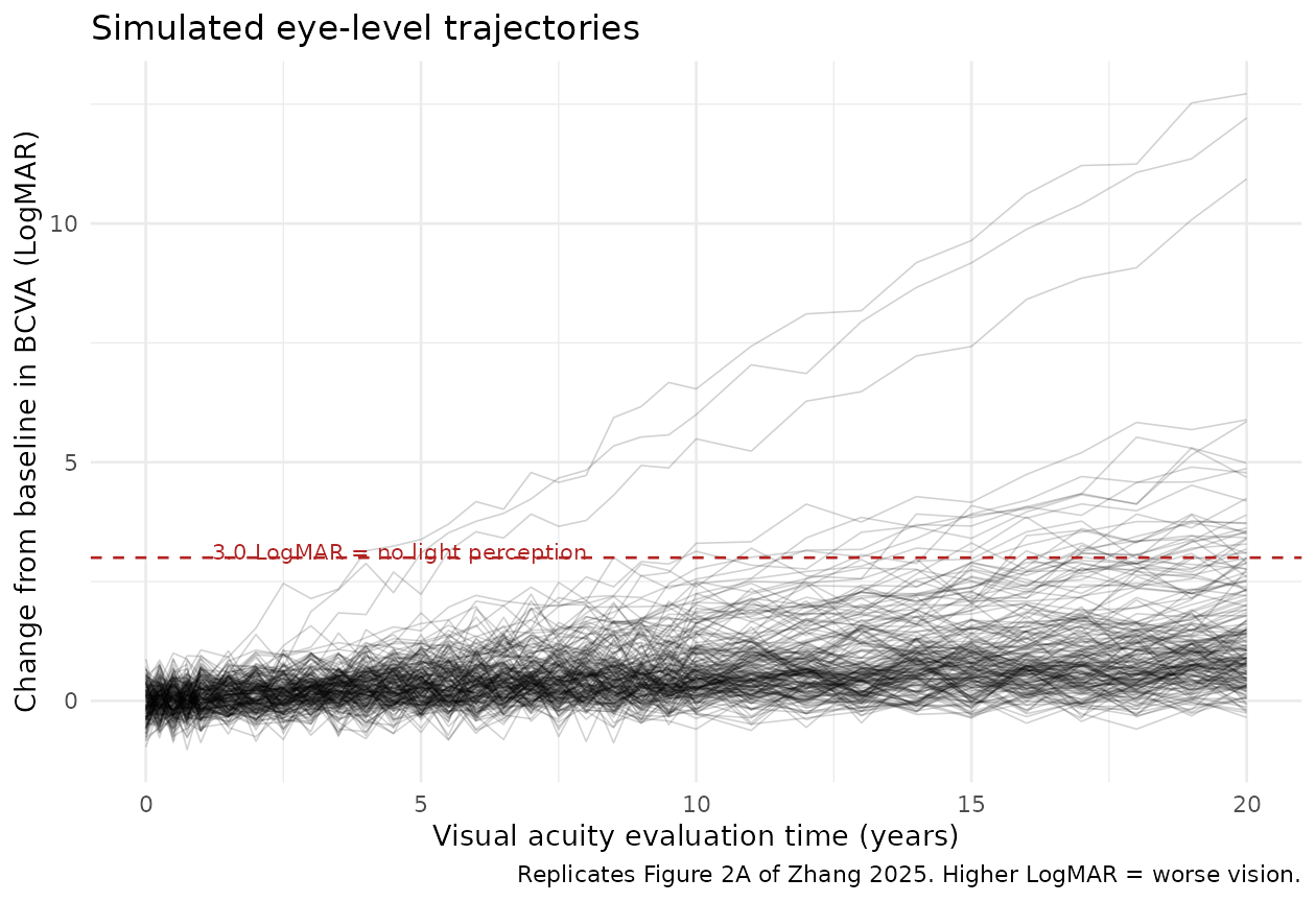
The dashed line marks 3.0 LogMAR, the scale ceiling that Zhang 2025 equates with no light perception. The packaged model does not impose that ceiling – see Assumptions and deviations.
Verification 4: visual predictive check against the published observed data
Supplement appendix 3 tabulates, for the whole cohort, the median, minimum and maximum observed change from baseline at each evaluation time along with the number of contributing study eyes. Those are real observed values extracted from the 14 source publications, so overlaying them on the model’s prediction interval is a genuine external check rather than a model-against-itself comparison.
observed <- tibble::tribble(
  ~time, ~median, ~min,   ~max,  ~n_eyes,
   0.25,  0.000, -0.28,  0.20,  36L,   # supplement appendix 3 row "<0.5", binned at 0.25
   0.75,  0.000, -0.26,  0.90,  38L,   # supplement appendix 3 row "0.5~1", binned at 0.75
   2.00,  0.000, -0.20,  1.90,  23L,
   3.00,  0.215, -0.04,  0.26,   4L,
   4.00,  0.365,  0.00,  1.70,  12L,
   5.00,  0.435,  0.00,  2.80,  18L,
   6.00,  0.160, -0.10,  2.29,  18L,
   7.00,  0.100, -0.30,  1.00,  16L,
   8.00,  0.375, -0.30,  2.50,  26L,
   9.00,  0.170,  0.00,  0.65,   8L,
  10.00,  0.425,  0.00,  2.08,  10L,
  11.00,  0.320,  0.08,  1.78,  13L,
  12.00,  0.440, -0.20,  2.68,  12L,
  13.00,  0.230,  0.00,  0.52,   7L,
  14.00,  0.735,  0.31,  2.70,   6L,
  15.00,  2.300,  1.23,  2.45,   3L,
  16.00,  0.550,  0.40,  2.68,   6L,
  18.00,  0.635,  0.57,  0.70,   2L,
  19.00,  0.485,  0.43,  0.53,   4L,
  20.00,  0.700,  0.48,  2.70,   9L,
  21.00,  1.000,  0.47,  3.00,   7L,
  22.00,  0.625,  0.47,  1.30,   4L,
  23.00,  2.950,  2.95,  2.95,   1L,
  24.00,  2.630,  2.63,  2.63,   1L,
  31.00,  3.000,  3.00,  3.00,   2L
)

# Fail loudly if the simulation grid and the observed table ever drift apart:
# a missing time would silently drop rows from the coverage check below.
stopifnot(all(observed$time %in% obs_t))
vpc_band <- sim_cohort |>
  dplyr::group_by(time) |>
  dplyr::summarise(
    Q05 = quantile(sim, 0.05),
    Q50 = quantile(sim, 0.50),
    Q95 = quantile(sim, 0.95),
    .groups = "drop"
  )

ggplot(vpc_band, aes(time, Q50)) +
  geom_ribbon(aes(ymin = Q05, ymax = Q95), alpha = 0.22, fill = "steelblue") +
  geom_line(linewidth = 0.8, colour = "steelblue") +
  geom_linerange(data = observed, inherit.aes = FALSE,
                 aes(x = time, ymin = min, ymax = max),
                 colour = "grey45", linewidth = 0.4) +
  geom_point(data = observed, inherit.aes = FALSE,
             aes(x = time, y = median, size = n_eyes)) +
  scale_size_area(max_size = 4, name = "Observed eyes") +
  labs(x = "Visual acuity evaluation time (years)",
       y = "Change from baseline in BCVA (LogMAR)",
       title = "Simulated 5th-50th-95th percentiles vs the published observed data",
       caption = paste("Band and line: packaged model,", n_eyes,
                       "simulated eyes. Points: observed medians (Zhang 2025 supplement appendix 3);",
                       "whiskers: observed min-max.")) +
  theme_minimal()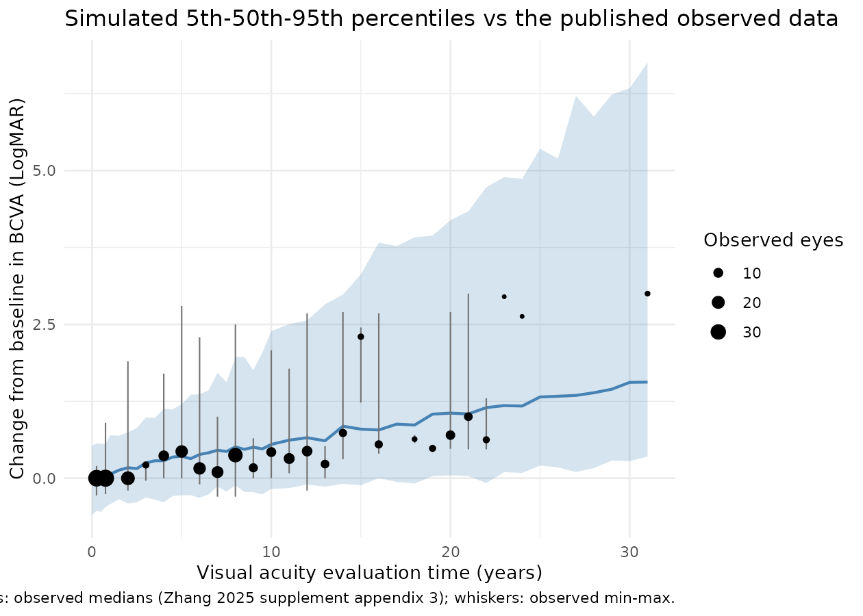
# Coverage of the observed medians by the simulated 5th-95th percentile band,
# restricted to evaluation times backed by at least 5 study eyes (a median over
# 1-4 eyes is not a stable statistic to check against).
coverage <- observed |>
  dplyr::filter(n_eyes >= 5) |>
  dplyr::left_join(vpc_band, by = "time") |>
  dplyr::mutate(inside = median >= Q05 & median <= Q95)

# Guard against a check that cannot go red: confirm rows exist and
# that every observed time matched a simulated time.
stopifnot(nrow(coverage) >= 15, !anyNA(coverage$Q50))

cover_frac <- mean(coverage$inside)

# Cohort-derived, so assert a bound that holds for ANY cohort this model can
# draw, not the value one run happened to give. The realised coverage is 1.00;
# 0.80 leaves room for the band edges to move with the draw while still going
# red if the model's slope or omega were badly mis-transcribed.
stopifnot(cover_frac >= 0.80)

cat("observed medians inside the simulated 5-95% band:",
    sum(coverage$inside), "of", nrow(coverage),
    sprintf("(%.0f%%)\n", 100 * cover_frac))
#> observed medians inside the simulated 5-95% band: 17 of 17 (100%)
A documented discordance: observed medians do not follow
K * t
The model’s median trajectory is slope_TV * t
(the median of
is 1), but the observed medians in supplement appendix 3 do not lie on
that line – they are 0.00 at 2 years, 0.365 at 4 years, 0.160 at 6 years
and 0.100 at 7 years. Regressing them through the origin gives a much
shallower slope than the fitted
:
obs_fit <- observed |> dplyr::filter(n_eyes >= 5)
obs_slope <- slope_through_origin(obs_fit$time, obs_fit$median)

cat(sprintf("origin-regression slope of the observed medians: %.4f LogMAR/year\n", obs_slope))
#> origin-regression slope of the observed medians: 0.0380 LogMAR/year
cat(sprintf("fitted typical K:                                %.4f LogMAR/year\n", 0.0566))
#> fitted typical K:                                0.0566 LogMAR/year
This is not a transcription error and it is not gated on. Each evaluation time in appendix 3 is contributed by a different subset of eyes – the studies have different follow-up lengths, and eyes observed at 6 years are not the eyes observed at 4 years – so the sequence of medians is not a longitudinal trajectory. The model was fitted to the individual longitudinal records, not to this table of cross-sectional summaries, and the two are only expected to agree in distribution (which the coverage check above confirms), not point by point.
Verification 5: subgroup trajectories
subgroup_sim <- groups |>
  dplyr::rowwise() |>
  dplyr::reframe(
    Group = Group,
    time  = published$time,
    Model = solve_typical_slope(`Published K`)
  )
#> ℹ change initial estimate of `lslope` to `-2.871746293773`
#> ℹ omega/sigma items treated as zero: 'etalslope'
#> ℹ change initial estimate of `lslope` to `-2.56915820223559`
#> ℹ omega/sigma items treated as zero: 'etalslope'
#> ℹ change initial estimate of `lslope` to `-2.32380872944567`
#> ℹ omega/sigma items treated as zero: 'etalslope'
#> ℹ change initial estimate of `lslope` to `-2.69562768110365`
#> ℹ omega/sigma items treated as zero: 'etalslope'
#> ℹ change initial estimate of `lslope` to `-2.41687423939617`
#> ℹ omega/sigma items treated as zero: 'etalslope'
#> ℹ change initial estimate of `lslope` to `-2.40794560865187`
#> ℹ omega/sigma items treated as zero: 'etalslope'

published_long <- groups |>
  dplyr::rowwise() |>
  dplyr::reframe(
    Group     = Group,
    time      = published$time,
    Published = published[[column]]
  )

dplyr::left_join(subgroup_sim, published_long, by = c("Group", "time")) |>
  ggplot(aes(time, Model, colour = Group)) +
  geom_line(linewidth = 0.8) +
  geom_point(aes(y = Published), size = 1.4) +
  labs(x = "Visual acuity evaluation time (years)",
       y = "Change from baseline in BCVA (LogMAR)",
       colour = "Group",
       title = "Post-hoc subgroup trajectories",
       caption = paste("Lines: packaged model with lslope overridden to each published post-hoc K.",
                       "Points: Zhang 2025 table 2 and supplement appendix 10.")) +
  theme_minimal() +
  theme(legend.position = "bottom", legend.direction = "vertical")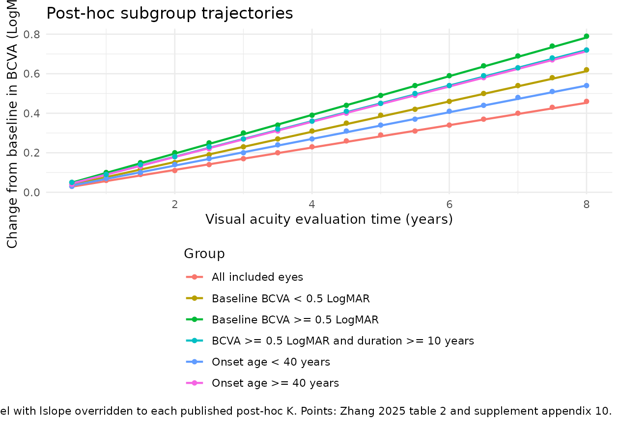
agreement <- dplyr::left_join(subgroup_sim, published_long,
                              by = c("Group", "time")) |>
  dplyr::mutate(diff = Model - Published)

stopifnot(nrow(agreement) == nrow(groups) * nrow(published), !anyNA(agreement$diff))

# Deterministic. Realised maximum is 0.0075 LogMAR across all six groups,
# driven by the two-decimal rounding of the published columns.
stopifnot(max(abs(agreement$diff)) < 0.012)

agreement |>
  dplyr::group_by(Group) |>
  dplyr::summarise(`Max |difference| (LogMAR)` = max(abs(diff)), .groups = "drop") |>
  knitr::kable(digits = 4,
caption = "Largest disagreement between the packaged model and each published simulation column, over 0.5-8 years.")| Group | Max |difference| (LogMAR) |
|---|---|
| All included eyes | 0.0072 |
| BCVA >= 0.5 LogMAR and duration >= 10 years | 0.0050 |
| Baseline BCVA < 0.5 LogMAR | 0.0072 |
| Baseline BCVA >= 0.5 LogMAR | 0.0068 |
| Onset age < 40 years | 0.0075 |
| Onset age >= 40 years | 0.0064 |
Clinical anchor: time to a clinically relevant change
The paper notes that the FDA regards a 15-letter change in visual acuity as clinically relevant; 15 ETDRS letters is 0.30 LogMAR. At the typical fitted rate this takes a little over five years, and at the fastest published subgroup rate about three.
tibble::tibble(
  Group = groups$Group,
  K     = groups$`Published K`
) |>
  dplyr::mutate(`Years to 0.30 LogMAR (15 ETDRS letters)` = 0.30 / K) |>
  dplyr::rename("K (LogMAR/year)" = K) |>
  knitr::kable(digits = c(0, 4, 1),
caption = "Time for the typical eye in each group to lose 15 ETDRS letters (0.30 LogMAR).")| Group | K (LogMAR/year) | Years to 0.30 LogMAR (15 ETDRS letters) |
|---|---|---|
| All included eyes | 0.0566 | 5.3 |
| Baseline BCVA < 0.5 LogMAR | 0.0766 | 3.9 |
| Baseline BCVA >= 0.5 LogMAR | 0.0979 | 3.1 |
| Onset age < 40 years | 0.0675 | 4.4 |
| Onset age >= 40 years | 0.0892 | 3.4 |
| BCVA >= 0.5 LogMAR and duration >= 10 years | 0.0900 | 3.3 |
Assumptions and deviations
-
No BCVA ceiling. Zhang 2025 codes no light
perception as 3.0 LogMAR and notes that “when the BCVA increased to 3
LogMAR, the eyes had no light perception, total blindness”. The
published structural model (
Effect = K x Time) has no ceiling, and none is imposed here, so simulations run long enough will predict changes above 3.0 LogMAR that are not physically attainable. Users simulating beyond roughly 30 years, or starting from an already-impaired baseline, should censor at the ceiling themselves. The model file reproduces the paper, not a corrected version of it. -
Monotone deterioration per eye. Because the
between-eye random effect is exponential,
slope_i = exp(lslope + etalslope)is strictly positive and no simulated eye can improve in its individual prediction. The observed improvements in the source data (changes from baseline as low as -0.30 LogMAR) are reproduced only through the additive residual error. This is the paper’s structure, not a simplification introduced here. - The random effect is between-EYE, and eyes are treated as independent. The analysis unit is the study eye (193 eyes from 117 patients), so both eyes of a bilaterally-affected patient enter as separate individuals. Zhang 2025 reports no patient-level or study-level random effect and no correlation structure between fellow eyes, so none is encoded. For a disease that is bilateral and genetically determined this almost certainly understates the effective correlation and therefore overstates the effective sample size; simulations intended to size a trial should treat the between-eye variance as a between-eye plus between-patient composite.
- No between-study variance. Despite being a meta-analysis, the model has no study-level term (see above). It cannot be used to explore between-study heterogeneity or to predict a new study’s mean.
-
Covariates are documented, not modelled. All eight
screened covariates were rejected (supplement appendix 6). Four with
existing canonical register names (
AGE,SCORE_BCVA,SEXF,RACE_ASIAN_NORTHEAST) are recorded in the model file’scovariatesDataExcludedmetadata; age at onset, disease duration, CYP4V2 genotype and family history have no canonical register entry and are described inpopulation$notesinstead. No new canonical covariate name was minted for a covariate that no model uses.-
SCORE_BCVAis defined in the covariate register on the ETDRS-letter scale (0-100, higher = better), whereas Zhang 2025 works in LogMAR (higher = worse). Because the covariate was screened out and is never referenced inmodel(), no scale reconciliation was required and none was performed; thecovariatesDataExcludedentry says so explicitly.
-
-
Subgroup slopes are post-hoc, not covariate
effects. The five subgroup
Kvalues are medians of individual empirical-Bayes estimates, obtained by Bayesian feedback after the final model was fixed. They are reproduced above by overridinglslope; they are deliberately not encoded as covariate effects in the model file, because no covariate reached significance and encoding them as such would misrepresent the paper. - Appendix 3 time binning. The first two rows of supplement appendix 3 are labelled “<0.5” and “0.5~1” rather than a single time. They are plotted at 0.25 and 0.75 years respectively. This affects only the observed-data overlay, not any parameter.
-
Observation-variable name. The observation is named
bcvacfb: the absolute-acuity statebcva(Mulyukov_2018_ranibizumab) with thecfbchange-from-baseline suffix, exactly asdas28cfbsits besidedas28. The register carried two competing forms for a change score when this model was written – thecfbsuffix and ad_<instrument>prefix (d_updrs,d_hr,d_rr,d_viral_load) – and the first draft of this model used the prefix form (d_bcva) on the strength of theLee_2011_parkinson_progressionanalogy. The maintainers ratified the suffix as the library-wide convention, sod_bcvawas renamed tobcvacfband the survivingd_-prefixed names are scheduled for conversion in a separate follow-up. Note that this model is algebraic with no absolute-acuity state of its own;bcvacfbis a change score throughout, and the covariate register’sSCORE_BCVAis on the ETDRS-letter scale (higher = better) rather than LogMAR, so the two are not interchangeable without conversion. -
Nothing is fixed. All three reported parameters
(
K,omega,sigma) were estimated, with RSEs and bootstrap confidence intervals given in supplement appendix 7, so nofixed()wrapper is used. -
Model 103 had a lower objective function.
Supplement appendix 4 records that model 103 (exponential IIV,
mixed additive-plus-proportional residual error) reached an
objective function of -323.382 against model 102’s -121.789, yet the
paper selected 102 as the base model and appendix 7 reports only an
additive
sigma. The packaged model follows the paper’s stated final model (102). The paper gives no rationale for preferring the higher-objective-function model; this is noted as a discrepancy in the source, not resolved here. - No NCA. This is a disease-progression model with no drug, no dose and no concentration, so PKNCA is not an applicable validation. The checks above are the closed-form, published-table-reproduction and visual-predictive-check patterns used for endogenous and mechanistic models.