COPD FEV1 combined aggregated + individual meta-analysis (Yang 2026)
Source:vignettes/articles/Yang_2026_copd_fev1.Rmd
Yang_2026_copd_fev1.RmdModel and source
Yang 2026 builds a combined aggregated-data + individual-patient-data (ADIPD) model of morning trough FEV1 in COPD, and in doing so builds two models that are packaged here separately:
Yang_2026_copd_fev1_ipd– the individual-patient-data model, fit to 2,241 patients in two fluticasone furoate / vilanterol trials.Yang_2026_copd_fev1_adipd_mbma– the combined model, fit to those individual records jointly with 4,137 arm-mean FEV1 observations from 296 published trials covering 23 compounds.Citation: Yang L, Llanos-Paez C, Yang S, Ambery C, Berges A, Kjellsson MC, Karlsson MO. A Combined Model-Based Meta-Analysis of Aggregated and Individual FEV1 Data From Randomized COPD Trials. CPT Pharmacometrics Syst Pharmacol. 2026;15(2):e70059. doi:10.1002/psp4.70059. Final parameter estimates are in Supporting Information Table S3; the model equations are in the Supporting Information section ‘NONMEM control stream for the combined ADIPD model’. The structural skeleton and the aggregated-data set are inherited from Llanos-Paez C, Ambery C, Yang S, Beerahee M, Plan EL, Karlsson MO. Joint longitudinal model-based meta-analysis of FEV1 and exacerbation rate in randomized COPD trials. J Pharmacokinet Pharmacodyn. 2023;50(4):297-314.
Article: https://doi.org/10.1002/psp4.70059
Supporting Information (Tables S1-S5 and both NONMEM control streams): https://europepmc.org/article/PMC/PMC12896389
ui_ipd   <- rxode2::rxode(readModelDb("Yang_2026_copd_fev1_ipd"))
#> ℹ parameter labels from comments will be replaced by 'label()'
ui_adipd <- rxode2::rxode(readModelDb("Yang_2026_copd_fev1_adipd_mbma"))
#> ℹ parameter labels from comments will be replaced by 'label()'
#> Warning: some etas defaulted to non-mu referenced, possible parsing error: eta_study_isv_cv_bd, eta_study_isv_cv_ai, eta_arm_base, etadps, etaeffref_vil
#> as a work-around try putting the mu-referenced expression on a simple line
Both models are purely algebraic – FEV1 is a
closed-form function of time and covariates, with no ODE states and no
PK layer. Drug effects are driven by per-arm total daily dose supplied
as CONMED_<drug>_DOSE covariate columns.
Population
The individual-patient data are the two 24-week, randomized, smoking-status stratified, placebo-controlled fluticasone furoate / vilanterol trials NCT01053988 (Kerwin 2013, n = 1025) and NCT01054885 (Martinez 2013, n = 1216), pooled to 2,241 patients: mean age 62 years (SD 8.8, range 40-85), 69.7% male, 54.2% current smokers, GOLD spirometric stage 2 in 46.5% / stage 3 in 44.1% / stage 4 in 8.66%, mean on-treatment FEV1 1.372 L (Supporting Information Table S1).
The aggregated data are the 4,137 arm-mean trough FEV1 observations from 298 studies of 250,543 patients assembled for the predecessor meta-analysis (Llanos-Paez 2023), covering 23 compounds in mono-, dual- and triple-therapy up to 24 November 2020. The two individual-patient studies are among those 298 and were removed from the aggregated side when fitting the combined model so that no observation contributes twice (paper Section 2.1). Arm sizes span 18 to 5,724 patients, which is what makes the central-limit-theorem approximation of Section 2.3.2 valid.
The same information is available programmatically:
pop <- ui_adipd$population
cat(paste0("* **", names(pop), "**: ", vapply(pop, paste, character(1), collapse = "; "), collapse = "\n"))- species: human
- n_subjects: 252784
- n_studies: 298
- age_range: Aggregated arm-mean ages across the published trials, pooled mean 63.4 years; the two individual-patient studies span 40-85 years with a mean of 62.
- age_median: 63.4 years (the pooled mean, used as the model’s centring constant)
- weight_range: not used as a model covariate
- sex_female_pct: 32.9
- disease_state: Chronic obstructive pulmonary disease across the GOLD spirometric severity range, in trials of mono-, dual- and triple-therapy with bronchodilators and anti-inflammatories. Endpoint is morning trough FEV1.
-
dose_range: Twenty-three compounds at their
clinically studied dose ranges, given as monotherapy, dual therapy or
triple therapy; see each CONMED_
_DOSE covariate entry for that drug’s reference dose. Placebo arms are encoded by all dose columns being zero. - regions: Multinational; the aggregated data are all published randomized COPD trials meeting the source analysis’s criteria up to 24 November 2020.
- trials_included: 298 studies in total. Aggregated data: 4,137 arm-mean trough FEV1 observations from 298 studies of 250,543 patients, inherited unchanged from the Llanos-Paez 2023 meta-analysis. Individual-patient data: NCT01053988 (n = 1025) and NCT01054885 (n = 1216), both 24-week fluticasone furoate / vilanterol trials. Those two studies were REMOVED from the aggregated data when fitting the combined model so that no observation contributes twice, leaving 296 aggregated studies alongside the 2 individual-patient studies.
- notes: n_subjects is the sum of the 250,543 aggregated patients and the 2,241 individual patients; because the two individual-patient studies are also among the 298 aggregated studies (and were excluded from the aggregated side to avoid duplication), this total counts each patient once. sex_female_pct is 1 - 0.671, using the pooled male fraction 0.671 that the source uses as its sex centring constant; the current-smoker fraction is correspondingly 0.463 and the mean GOLD stage 3. Study durations run from short trials to 19 studies longer than 52 weeks (Supporting Information Figure S4C). The paper reports a between-study shrinkage of 43.4% on the disease-progression slope random effect, so study-level disease-progression draws are weakly informed.
Source trace
Each ini() entry in the two model files carries an
in-file comment naming its source location. The table below collects the
structural origins.
| Model component | Source location |
|---|---|
Overall structure
FEV1 = B + PBO - DP + E + PostBD correction + err
|
Paper Equation 10 (Section 2.4) |
| Individual-patient parameter values | Supporting Information Table S2 |
| Combined-model parameter values | Supporting Information Table S3 |
| Individual-patient model equations | Supporting Information, “NONMEM control stream for the IPD model” |
| Combined-model equations | Supporting Information, “NONMEM control stream for the combined ADIPD model” |
| Covariate relationships retained per model | Supporting Information Table S4 |
| Normal approximation to the arm-mean of a log-normal | Paper Section 2.3.2, Equations 1-8 |
| Linearization of the placebo mixture, the baseline step function and the severity covariate | Paper Section 2.3.1 |
| Post-SABD reversibility shift of 0.18 L | Paper Section 2.4, note following Equation 10 |
Aggregated residual error scaled by 1/sqrt(N)
|
Paper Equation 10, err = eps_AD / sqrt(N_ij)
|
Individual-patient-model values are taken from Table
S2, not from that control stream’s $THETA records,
which carry that run’s initial estimates (1.18 vs the final
1.17 for baseline, and similar small differences elsewhere).
Combined-model values are taken from the control stream’s
$THETA, whose converged values agree with Table S3 to every
displayed digit while carrying more precision (1.06908 vs the tabulated
1.07).
n_par <- function(ui) sum(!is.na(ui$iniDf$ntheta))
n_eta <- function(ui) sum(!is.na(ui$iniDf$neta1))
data.frame(
  Model = c("Yang_2026_copd_fev1_ipd", "Yang_2026_copd_fev1_adipd_mbma"),
  `Fixed effects` = c(n_par(ui_ipd), n_par(ui_adipd)),
  `Random effects` = c(n_eta(ui_ipd), n_eta(ui_adipd)),
  check.names = FALSE
) |> knitr::kable()| Model | Fixed effects | Random effects |
|---|---|---|
| Yang_2026_copd_fev1_ipd | 18 | 4 |
| Yang_2026_copd_fev1_adipd_mbma | 67 | 15 |
Simulation helpers
Neither model consumes rxode2 dose events, so an event table is
simply a frame of observation rows carrying the covariate columns.
evid = 0 throughout.
ipd_covs <- function(age = 62, sexf = 0, smoke = 1, gold = 3, vi = 0, ff = 0) {
  list(AGE = age, SEXF = sexf, SMOKE = smoke, DIS_COPD_GOLD = gold,
       CONMED_VILANTEROL_DOSE = vi, CONMED_FLUTICASONEFUROATE_DOSE = ff)
}

# Every CONMED_<drug>_DOSE column the combined model reads, defaulted to zero
# (an all-zero row is a placebo / background-therapy-only arm).
adipd_drugs <- c(
  "ACLIDINIUM", "ARFORMOTEROL", "AZD9668", "BATEFENTEROL", "BEA2180",
  "BECLOMETHASONE", "BUDESONIDE", "CILOMILAST", "FLUTICASONEFUROATE",
  "FLUTICASONEPROPIONATE", "FORMOTEROL", "GLYCOPYRRONIUM", "GSK233705",
  "INDACATEROL", "MOMETASONE", "OLODATEROL", "PH797804", "REVEFENACIN",
  "ROFLUMILAST", "SALMETEROL", "TIOTROPIUM", "UMECLIDINIUM", "VILANTEROL"
)

adipd_covs <- function(...) {
  base <- as.list(setNames(rep(0, length(adipd_drugs)),
                           paste0("CONMED_", adipd_drugs, "_DOSE")))
  base <- c(base, list(
    FORM_ACLIDINIUM_BID = 0, FORM_MOMETASONE_BID = 0, FORM_OLODATEROL_BID = 0,
    FORM_BATEFENTEROL_BID = 0, FORM_TIOTROPIUM_SMI = 0,
    FORM_TIOTROPIUM_OPENLABEL = 0,
    # Reference arm: aggregated record, reference covariate values, no
    # background therapy, no reconciliation term.
    DTYPE_AGGREGATED = 1, N_ARM = 200, MEAS_POSTBD = 0, FEV1_PBD_ANCHOR = 0,
    OCS_NONRESPONDER = 0, INCL_EXAC_REQUIRED = 0,
    AGE = 63.4, SEXF = 0.329, SMOKE = 0.463, DIS_COPD_GOLD = 3,
    DIS_COPD_GOLD_LOW = 2, DIS_COPD_GOLD_HIGH = 4,
    BGTHER_ICS_RUNIN_PCT = 0, BGTHER_LABA_RUNIN_PCT = 0,
    BGTHER_LAAC_RUNIN_PCT = 0, BGTHER_ICS_MAINT_PCT = 0,
    BGTHER_LABA_MAINT_PCT = 0, BGTHER_LAAC_MAINT_PCT = 0))
  mods <- list(...)
  for (n in names(mods)) base[[n]] <- mods[[n]]
  base
}

make_events <- function(covs_list, times) {
  do.call(rbind, lapply(seq_along(covs_list), function(i) {
    cbind(data.frame(id = i, time = times, evid = 0L, amt = NA_real_),
          as.data.frame(covs_list[[i]]))
  }))
}

# zeroRe() gives the typical-value prediction with every random effect at zero.
solve_typical <- function(ui, ev, ...) {
  rxode2::rxSolve(rxode2::zeroRe(ui), ev, returnType = "data.frame", ...)
}
Check 1 – the individual-patient model reproduces its closed form exactly
The individual-patient model is small enough to write out independently. Because both sides use the same parameter values and no random draw is involved, this is a pure numerical-identity check and a tight bound is the correct assertion.
closed_form_ipd <- function(t, age, sexf, smoke, gold, vi, ff) {
  b <- 1.17 *
    (1 - 0.0144 * (age - 62)) *
    (1 + ifelse(gold <= 3, -0.47, -0.368) * (gold - 3)) *
    (1 - 0.0419 * (1 - smoke)) *
    (1 - 0.248 * sexf)
  dp <- 0.0241 * (1 - 1.89 * (gold - 3)) * t / 52
  ed50_vi <- exp(0.709); ed50_ff <- exp(2.43)
  emax_vi <- 0.117 / 25 * (ed50_vi + 25) *
    (1 - 0.0119 * (age - 62)) *
    (1 + ifelse(gold <= 3, -0.163, -0.533) * (gold - 3))
  emax_ff <- 0.0304 / 100 * (ed50_ff + 100)
  b - dp + (t > 0) * (emax_vi * vi / (vi + ed50_vi) + emax_ff * ff / (ff + ed50_ff))
}

grid_ipd <- expand.grid(
  age = c(45, 62, 78), sexf = c(0, 1), smoke = c(0, 1),
  gold = c(2, 3, 4), vi = c(0, 25), ff = c(0, 50, 100, 200)
)
ev_ipd <- make_events(
  lapply(seq_len(nrow(grid_ipd)), function(i) {
    with(grid_ipd[i, ], ipd_covs(age, sexf, smoke, gold, vi, ff))
  }),
  times = c(0, 4, 12, 24)
)
sim_ipd <- solve_typical(ui_ipd, ev_ipd)
#> ℹ omega/sigma items treated as zero: 'etabase', 'etadps', 'etaeffref_vi', 'etapowSd_FEV1'
#> Warning: multi-subject simulation without without 'omega'

expected_ipd <- closed_form_ipd(
  sim_ipd$time, sim_ipd$AGE, sim_ipd$SEXF, sim_ipd$SMOKE, sim_ipd$DIS_COPD_GOLD,
  sim_ipd$CONMED_VILANTEROL_DOSE, sim_ipd$CONMED_FLUTICASONEFUROATE_DOSE
)
max_abs_err <- max(abs(sim_ipd$FEV1 - expected_ipd))
cat(sprintf("%d covariate/time combinations; max |solve - closed form| = %.3e L\n",
            nrow(sim_ipd), max_abs_err))
#> 1152 covariate/time combinations; max |solve - closed form| = 0.000e+00 L

# Deterministic identity: both sides are the same algebra on the same numbers,
# so the only difference possible is floating-point rounding.
stopifnot(nrow(sim_ipd) > 500, max_abs_err < 1e-10)
Check 2 – reference-dose efficacies are recovered exactly
The source parameterises each dose-response drug by its effect
at a reference dose rather than by Emax, via
Emax = EffRef / RefDose * (ED50 + RefDose). Giving exactly
the reference dose must therefore return exactly the published reference
efficacy. This is the check that catches a mis-transcribed ED50, a
mis-transcribed reference dose, or a units slip between the two – all of
which would leave the model solving happily while predicting the wrong
effect.
ev_ref <- make_events(list(
  ipd_covs(),                     # placebo
  ipd_covs(vi = 25),              # vilanterol at its 25 ug/day reference dose
  ipd_covs(ff = 100)              # fluticasone furoate at its 100 ug/day reference
), times = c(0, 24))
sim_ref <- solve_typical(ui_ipd, ev_ref)
#> ℹ omega/sigma items treated as zero: 'etabase', 'etadps', 'etaeffref_vi', 'etapowSd_FEV1'
#> Warning: multi-subject simulation without without 'omega'
wk24 <- sim_ref[sim_ref$time == 24, ]

ipd_ref_tab <- data.frame(
  Drug = c("Vilanterol 25 ug/day", "Fluticasone furoate 100 ug/day"),
  `Published reference efficacy (L)` = c(0.117, 0.0304),
  `Simulated effect vs placebo (L)` = round(wk24$FEV1[2:3] - wk24$FEV1[1], 6),
  check.names = FALSE
)
knitr::kable(ipd_ref_tab)| Drug | Published reference efficacy (L) | Simulated effect vs placebo (L) |
|---|---|---|
| Vilanterol 25 ug/day | 0.1170 | 0.1170 |
| Fluticasone furoate 100 ug/day | 0.0304 | 0.0304 |
The combined model applies one further multiplier before the effect
reaches the prediction: the predicted baseline scales the bronchodilator
and anti-inflammatory effects through rel_bd and
rel_ai. At the reference covariate values the arm-mean
baseline is below the 1.2 L centring point, so every drug’s effect is
attenuated by the same factor – which makes the identity below an exact
test of all 13 dose-response drugs at once.
Six of the 13 also carry a class effect-onset time course, which is still a fraction of a percent short of its plateau at week 24. That factor is read back from the solve rather than assumed to be 1, so the identity below simultaneously checks each drug’s reference efficacy, its ED50, its reference dose and its onset rate.
ref_doses <- list(
  ACLIDINIUM        = list(dose = 200, effref = 0.075184,  cls = "bd", tc = NA),
  BUDESONIDE        = list(dose = 320, effref = 0.0336889, cls = "ai", tc = "tc_ics"),
  FORMOTEROL        = list(dose = 18,  effref = 0.0699607, cls = "bd", tc = NA),
  INDACATEROL       = list(dose = 75,  effref = 0.12618,   cls = "bd", tc = "tc_laba"),
  GLYCOPYRRONIUM    = list(dose = 100, effref = 0.12743,   cls = "bd", tc = "tc_laac"),
  ROFLUMILAST       = list(dose = 500, effref = 0.0811084, cls = "ai", tc = "tc_pde4"),
  TIOTROPIUM        = list(dose = 18,  effref = 0.122236,  cls = "bd", tc = "tc_laac"),
  VILANTEROL        = list(dose = 25,  effref = 0.109036,  cls = "bd", tc = NA),
  REVEFENACIN       = list(dose = 175, effref = 0.148945,  cls = "bd", tc = NA),
  OLODATEROL        = list(dose = 5,   effref = 0.0889892, cls = "bd", tc = NA),
  BATEFENTEROL      = list(dose = 400, effref = 0.195297,  cls = "bd", tc = NA),
  FLUTICASONEFUROATE = list(dose = 100, effref = 0.0400295, cls = "ai", tc = NA)
)

ev_adipd_ref <- make_events(
  c(list(adipd_covs()),
    lapply(names(ref_doses), function(d) {
      a <- list(); a[[paste0("CONMED_", d, "_DOSE")]] <- ref_doses[[d]]$dose
      do.call(adipd_covs, a)
    })),
  times = c(0, 24)
)
sim_adipd_ref <- solve_typical(ui_adipd, ev_adipd_ref)
#> Warning: No sigma parameters in the model
#> Warning: some etas defaulted to non-mu referenced, possible parsing error: eta_study_isv_cv_bd, eta_study_isv_cv_ai, eta_arm_base, etadps, etaeffref_vil
#> as a work-around try putting the mu-referenced expression on a simple line
#> ℹ omega/sigma items treated as zero: 'eta_study_base', 'eta_study_dps', 'eta_study_pmx', 'eta_study_isv_cv_bd', 'eta_study_isv_cv_ai', 'eta_study_age', 'eta_study_smoke', 'eta_study_bgics', 'eta_study_bglaba', 'eta_study_bglaac', 'eta_arm_base', 'etabase', 'etadps', 'etaeffref_vil', 'etapowSd_FEV1'
#> Warning: multi-subject simulation without without 'omega'
w24 <- sim_adipd_ref[sim_adipd_ref$time == 24, ]

# rel_bd / rel_ai are model outputs, so the expected value is read from the
# solve rather than hand-recomputed.
rel_bd <- w24$rel_bd[1]; rel_ai <- w24$rel_ai[1]
tc_at_24 <- function(nm) if (is.na(nm)) 1 else w24[[nm]][1]

adipd_ref_tab <- data.frame(
  Drug = names(ref_doses),
  `Reference dose (ug/day)` = vapply(ref_doses, function(x) x$dose, numeric(1)),
  `Published reference efficacy (L)` = vapply(ref_doses, function(x) x$effref, numeric(1)),
  `Onset fraction at week 24` = vapply(ref_doses, function(x) tc_at_24(x$tc), numeric(1)),
  `Expected effect (L)` = vapply(ref_doses, function(x)
    x$effref * tc_at_24(x$tc) * if (x$cls == "bd") rel_bd else rel_ai, numeric(1)),
  `Simulated effect vs placebo (L)` = w24$FEV1[-1] - w24$FEV1[1],
  check.names = FALSE, row.names = NULL
)
knitr::kable(adipd_ref_tab, digits = 6)| Drug | Reference dose (ug/day) | Published reference efficacy (L) | Onset fraction at week 24 | Expected effect (L) | Simulated effect vs placebo (L) |
|---|---|---|---|---|---|
| ACLIDINIUM | 200 | 0.075184 | 1.000000 | 0.072071 | 0.072071 |
| BUDESONIDE | 320 | 0.033689 | 0.999906 | 0.031541 | 0.031541 |
| FORMOTEROL | 18 | 0.069961 | 1.000000 | 0.067064 | 0.067064 |
| INDACATEROL | 75 | 0.126180 | 1.000000 | 0.120955 | 0.120955 |
| GLYCOPYRRONIUM | 100 | 0.127430 | 1.000000 | 0.122153 | 0.122153 |
| ROFLUMILAST | 500 | 0.081108 | 0.999906 | 0.075937 | 0.075937 |
| TIOTROPIUM | 18 | 0.122236 | 1.000000 | 0.117174 | 0.117174 |
| VILANTEROL | 25 | 0.109036 | 1.000000 | 0.104521 | 0.104521 |
| REVEFENACIN | 175 | 0.148945 | 1.000000 | 0.142777 | 0.142777 |
| OLODATEROL | 5 | 0.088989 | 1.000000 | 0.085304 | 0.085304 |
| BATEFENTEROL | 400 | 0.195297 | 1.000000 | 0.187209 | 0.187209 |
| FLUTICASONEFUROATE | 100 | 0.040030 | 1.000000 | 0.037481 | 0.037481 |
cat(sprintf("Baseline scaling at the reference arm: rel_bd = %.6f, rel_ai = %.6f\n",
            rel_bd, rel_ai))
#> Baseline scaling at the reference arm: rel_bd = 0.958589, rel_ai = 0.936323
stopifnot(
  nrow(adipd_ref_tab) == 12L,
  max(abs(adipd_ref_tab[["Simulated effect vs placebo (L)"]] -
            adipd_ref_tab[["Expected effect (L)"]])) < 1e-9
)
Tiotropium via the Respimat soft-mist inhaler is the one dose-response whose ED50 is derived rather than estimated, so it is checked separately at its own 5 ug/day reference dose.
ev_smi <- make_events(list(
  adipd_covs(),
  adipd_covs(CONMED_TIOTROPIUM_DOSE = 5, FORM_TIOTROPIUM_SMI = 1),
  adipd_covs(CONMED_TIOTROPIUM_DOSE = 18, FORM_TIOTROPIUM_OPENLABEL = 1)
), times = c(0, 24))
s_smi <- solve_typical(ui_adipd, ev_smi)
#> Warning: No sigma parameters in the model
#> Warning: some etas defaulted to non-mu referenced, possible parsing error: eta_study_isv_cv_bd, eta_study_isv_cv_ai, eta_arm_base, etadps, etaeffref_vil
#> as a work-around try putting the mu-referenced expression on a simple line
#> ℹ omega/sigma items treated as zero: 'eta_study_base', 'eta_study_dps', 'eta_study_pmx', 'eta_study_isv_cv_bd', 'eta_study_isv_cv_ai', 'eta_study_age', 'eta_study_smoke', 'eta_study_bgics', 'eta_study_bglaba', 'eta_study_bglaac', 'eta_arm_base', 'etabase', 'etadps', 'etaeffref_vil', 'etapowSd_FEV1'
#> Warning: multi-subject simulation without without 'omega'
w_smi <- s_smi[s_smi$time == 24, ]
eff_smi <- w_smi$FEV1[2] - w_smi$FEV1[1]
eff_ol  <- w_smi$FEV1[3] - w_smi$FEV1[1]
tc_laac_24 <- w_smi$tc_laac[1]

cat(sprintf("Respimat 5 ug/day:    simulated %.6f L, expected %.6f L\n",
            eff_smi, 0.120457 * tc_laac_24 * rel_bd))
#> Respimat 5 ug/day:    simulated 0.115469 L, expected 0.115469 L
cat(sprintf("Open-label 18 ug/day: simulated %.6f L, expected %.6f L (0.918377 x blinded)\n",
            eff_ol, 0.918377 * 0.122236 * tc_laac_24 * rel_bd))
#> Open-label 18 ug/day: simulated 0.107610 L, expected 0.107610 L (0.918377 x blinded)
stopifnot(
  abs(eff_smi - 0.120457 * tc_laac_24 * rel_bd) < 1e-9,
  abs(eff_ol - 0.918377 * 0.122236 * tc_laac_24 * rel_bd) < 1e-9
)
Check 3 – covariate directions match Table S4
Supporting Information Table S4 tabulates which covariate relationships each model retained and in which direction. The signs below are read off the packaged models by perturbing one covariate at a time from the reference arm.
delta_ipd <- function(mod_args, t = 24) {
  ev <- make_events(list(do.call(ipd_covs, list()),
                         do.call(ipd_covs, mod_args)), times = c(0, t))
  s <- solve_typical(ui_ipd, ev)
  s$FEV1[s$time == t][2] - s$FEV1[s$time == t][1]
}

sign_tab <- data.frame(
  Covariate = c("Age +10 years", "GOLD stage 3 -> 4", "Non-current smoker",
                "Female sex"),
  `Change in FEV1 (L)` = c(
    delta_ipd(list(age = 72)),
    delta_ipd(list(gold = 4)),
    delta_ipd(list(smoke = 0)),
    delta_ipd(list(sexf = 1))
  ),
  `Table S4 direction` = rep("negative on baseline", 4),
  check.names = FALSE
)
#> ℹ omega/sigma items treated as zero: 'etabase', 'etadps', 'etaeffref_vi', 'etapowSd_FEV1'
#> Warning: multi-subject simulation without without 'omega'
#> ℹ omega/sigma items treated as zero: 'etabase', 'etadps', 'etaeffref_vi', 'etapowSd_FEV1'
#> Warning: multi-subject simulation without without 'omega'
#> ℹ omega/sigma items treated as zero: 'etabase', 'etadps', 'etaeffref_vi', 'etapowSd_FEV1'
#> Warning: multi-subject simulation without without 'omega'
#> ℹ omega/sigma items treated as zero: 'etabase', 'etadps', 'etaeffref_vi', 'etapowSd_FEV1'
#> Warning: multi-subject simulation without without 'omega'
knitr::kable(sign_tab, digits = 4)| Covariate | Change in FEV1 (L) | Table S4 direction |
|---|---|---|
| Age +10 years | -0.1685 | negative on baseline |
| GOLD stage 3 -> 4 | -0.4095 | negative on baseline |
| Non-current smoker | -0.0490 | negative on baseline |
| Female sex | -0.2902 | negative on baseline |
# All four are documented NEGATIVE relationships in Table S4, and all four are
# deterministic typical-value differences, so an exact sign test is valid here
# (contrast with a cohort-derived sign, which would not be).
stopifnot(all(sign_tab[[2]] < 0))
The combined model additionally retains a positive effect of the predicted baseline on both drug-effect classes, and an exacerbation-history entry criterion on baseline. Higher baseline must therefore give a larger drug effect.
eff_at_gold <- function(gold_low, gold_high) {
  ev <- make_events(list(
    adipd_covs(DIS_COPD_GOLD_LOW = gold_low, DIS_COPD_GOLD_HIGH = gold_high),
    adipd_covs(DIS_COPD_GOLD_LOW = gold_low, DIS_COPD_GOLD_HIGH = gold_high,
               CONMED_TIOTROPIUM_DOSE = 18)
  ), times = c(0, 24))
  s <- solve_typical(ui_adipd, ev)
  w <- s[s$time == 24, ]
  c(baseline = s$FEV1[s$time == 0][1], effect = w$FEV1[2] - w$FEV1[1])
}
milder  <- eff_at_gold(1, 3)   # mean stage 2
#> Warning: No sigma parameters in the model
#> Warning: some etas defaulted to non-mu referenced, possible parsing error: eta_study_isv_cv_bd, eta_study_isv_cv_ai, eta_arm_base, etadps, etaeffref_vil
#> as a work-around try putting the mu-referenced expression on a simple line
#> ℹ omega/sigma items treated as zero: 'eta_study_base', 'eta_study_dps', 'eta_study_pmx', 'eta_study_isv_cv_bd', 'eta_study_isv_cv_ai', 'eta_study_age', 'eta_study_smoke', 'eta_study_bgics', 'eta_study_bglaba', 'eta_study_bglaac', 'eta_arm_base', 'etabase', 'etadps', 'etaeffref_vil', 'etapowSd_FEV1'
#> Warning: multi-subject simulation without without 'omega'
severer <- eff_at_gold(3, 4)   # mean stage 3.5
#> Warning: No sigma parameters in the model
#> some etas defaulted to non-mu referenced, possible parsing error: eta_study_isv_cv_bd, eta_study_isv_cv_ai, eta_arm_base, etadps, etaeffref_vil
#> as a work-around try putting the mu-referenced expression on a simple line
#> ℹ omega/sigma items treated as zero: 'eta_study_base', 'eta_study_dps', 'eta_study_pmx', 'eta_study_isv_cv_bd', 'eta_study_isv_cv_ai', 'eta_study_age', 'eta_study_smoke', 'eta_study_bgics', 'eta_study_bglaba', 'eta_study_bglaac', 'eta_arm_base', 'etabase', 'etadps', 'etaeffref_vil', 'etapowSd_FEV1'
#> Warning: multi-subject simulation without without 'omega'

data.frame(
  Cohort = c("Milder (mean GOLD 2)", "More severe (mean GOLD 3.5)"),
  `Baseline FEV1 (L)` = c(milder[["baseline"]], severer[["baseline"]]),
  `Tiotropium 18 ug/day effect (L)` = c(milder[["effect"]], severer[["effect"]]),
  check.names = FALSE
) |> knitr::kable(digits = 4)| Cohort | Baseline FEV1 (L) | Tiotropium 18 ug/day effect (L) |
|---|---|---|
| Milder (mean GOLD 2) | 1.5415 | 0.1394 |
| More severe (mean GOLD 3.5) | 0.8785 | 0.1060 |
stopifnot(
  milder[["baseline"]] > severer[["baseline"]],   # higher severity, lower baseline
  milder[["effect"]]   > severer[["effect"]]      # higher baseline, larger effect
)
Check 4 – the aggregation-bias correction (paper Figure 2 and Section 3.2)
This is the paper’s central methodological claim, and it is the reason the combined model’s typical baseline is 1.07 L where the aggregated-data-only model reported 1.17 L (paper Section 4).
An individual baseline is log-normal about the study typical value.
The arm mean of N such baselines is
not log-normal: by the central limit theorem it is
approximately normal, centred on the log-normal’s mean
theta * exp(omega^2 / 2) rather than on its median
theta, with standard deviation shrunk by
sqrt(N). Fitting an aggregated arm mean as though it were
log-normal about theta therefore forces theta
upward.
The check below compares the packaged model’s encoded approximation against a brute-force Monte Carlo of the actual arm mean.
set.seed(20260912)
cv_base <- ui_adipd$theta[["cv_base"]]
theta_b <- ui_adipd$theta[["base"]]

# What the model predicts for an aggregated arm mean at the reference arm.
model_arm_mean <- solve_typical(
  ui_adipd, make_events(list(adipd_covs(N_ARM = 200)), times = 0)
)$FEV1[1]
#> Warning: No sigma parameters in the model
#> Warning: some etas defaulted to non-mu referenced, possible parsing error: eta_study_isv_cv_bd, eta_study_isv_cv_ai, eta_arm_base, etadps, etaeffref_vil
#> as a work-around try putting the mu-referenced expression on a simple line
#> ℹ omega/sigma items treated as zero: 'eta_study_base', 'eta_study_dps', 'eta_study_pmx', 'eta_study_isv_cv_bd', 'eta_study_isv_cv_ai', 'eta_study_age', 'eta_study_smoke', 'eta_study_bgics', 'eta_study_bglaba', 'eta_study_bglaac', 'eta_arm_base', 'etabase', 'etadps', 'etaeffref_vil', 'etapowSd_FEV1'

# Brute force: draw 200 individual log-normal baselines per arm, 20000 arms.
n_arm <- 200L; n_rep <- 20000L
arm_means <- colMeans(matrix(
  theta_b * exp(rnorm(n_arm * n_rep, 0, cv_base)), nrow = n_arm))

agg_tab <- data.frame(
  Quantity = c("Individual median (theta)",
               "Model's aggregated arm mean",
               "Monte-Carlo mean of the arm mean",
               "Model's arm-mean SD at N = 200",
               "Monte-Carlo SD of the arm mean"),
  Value = c(
    theta_b,
    model_arm_mean,
    mean(arm_means),
    theta_b * sqrt(exp(cv_base^2) - 1) * exp(cv_base^2 / 2) / sqrt(n_arm),
    sd(arm_means)
  )
)
knitr::kable(agg_tab, digits = 5)| Quantity | Value |
|---|---|
| Individual median (theta) | 1.06908 |
| Model’s aggregated arm mean | 1.09952 |
| Monte-Carlo mean of the arm mean | 1.09950 |
| Model’s arm-mean SD at N = 200 | 0.01868 |
| Monte-Carlo SD of the arm mean | 0.01868 |
rel_err_mean <- abs(mean(arm_means) - model_arm_mean) / model_arm_mean
rel_err_sd   <- abs(sd(arm_means) -
                      theta_b * sqrt(exp(cv_base^2) - 1) *
                      exp(cv_base^2 / 2) / sqrt(n_arm)) / sd(arm_means)
cat(sprintf("Relative error vs Monte Carlo: mean %.4f%%, SD %.3f%%\n",
            100 * rel_err_mean, 100 * rel_err_sd))
#> Relative error vs Monte Carlo: mean 0.0020%, SD 0.008%

# 20000 replicates of a mean-of-200 gives a Monte-Carlo standard error of about
# 0.012% on the mean and about 0.5% on the SD, so these bounds sit several
# Monte-Carlo standard errors outside the noise while still failing loudly if
# the exp(omega^2/2) factor or the sqrt(N) shrinkage were dropped (either of
# which moves these by 2.8% and 100% respectively).
stopifnot(rel_err_mean < 0.005, rel_err_sd < 0.05)

# The uncorrected alternative -- treating the arm mean as log-normal about the
# MEDIAN with SD/sqrt(N) -- is biased low by exactly exp(omega^2/2).
bias <- (model_arm_mean - theta_b) / theta_b
cat(sprintf("Uncorrected log-normal arm mean would sit %.2f%% below the true mean.\n",
            100 * bias))
#> Uncorrected log-normal arm mean would sit 2.85% below the true mean.
stopifnot(abs(bias - (exp(cv_base^2 / 2) - 1)) < 1e-10)
The 2.8% offset recovered here is the mechanism; the paper’s own SSE found an 8-10% bias on the baseline typical value and its variance (Section 3.2, Figure 3A) because there the estimator absorbs the discrepancy over a whole data set rather than at a single arm.
Check 5 – the aggregated residual error shrinks as
1/sqrt(N)
narm_grid <- c(18, 50, 200, 1000, 5724)   # the paper's reported arm-size range
ev_narm <- make_events(lapply(narm_grid, function(n) adipd_covs(N_ARM = n)),
                       times = 24)
s_narm <- solve_typical(ui_adipd, ev_narm)
#> Warning: No sigma parameters in the model
#> Warning: some etas defaulted to non-mu referenced, possible parsing error: eta_study_isv_cv_bd, eta_study_isv_cv_ai, eta_arm_base, etadps, etaeffref_vil
#> as a work-around try putting the mu-referenced expression on a simple line
#> ℹ omega/sigma items treated as zero: 'eta_study_base', 'eta_study_dps', 'eta_study_pmx', 'eta_study_isv_cv_bd', 'eta_study_isv_cv_ai', 'eta_study_age', 'eta_study_smoke', 'eta_study_bgics', 'eta_study_bglaba', 'eta_study_bglaac', 'eta_arm_base', 'etabase', 'etadps', 'etaeffref_vil', 'etapowSd_FEV1'
#> Warning: multi-subject simulation without without 'omega'

resid_tab <- data.frame(
  `Arm size N` = narm_grid,
  `Residual SD (L)` = s_narm$sdFEV1,
  `addSd / sqrt(N)` = ui_adipd$theta[["addSd_FEV1"]] / sqrt(narm_grid),
  check.names = FALSE
)
knitr::kable(resid_tab, digits = 5)| Arm size N | Residual SD (L) | addSd / sqrt(N) |
|---|---|---|
| 18 | 0.04758 | 0.04758 |
| 50 | 0.02855 | 0.02855 |
| 200 | 0.01427 | 0.01427 |
| 1000 | 0.00638 | 0.00638 |
| 5724 | 0.00267 | 0.00267 |
An individual-patient record instead carries the power error model, whose SD rises with the prediction.
ev_dt <- make_events(list(adipd_covs(DTYPE_AGGREGATED = 0, N_ARM = 1)),
                     times = c(0, 24))
s_dt <- solve_typical(ui_adipd, ev_dt)
#> Warning: No sigma parameters in the model
#> Warning: some etas defaulted to non-mu referenced, possible parsing error: eta_study_isv_cv_bd, eta_study_isv_cv_ai, eta_arm_base, etadps, etaeffref_vil
#> as a work-around try putting the mu-referenced expression on a simple line
#> ℹ omega/sigma items treated as zero: 'eta_study_base', 'eta_study_dps', 'eta_study_pmx', 'eta_study_isv_cv_bd', 'eta_study_isv_cv_ai', 'eta_study_age', 'eta_study_smoke', 'eta_study_bgics', 'eta_study_bglaba', 'eta_study_bglaac', 'eta_arm_base', 'etabase', 'etadps', 'etaeffref_vil', 'etapowSd_FEV1'
expected_sd <- ui_adipd$theta[["powSd_FEV1"]] *
  s_dt$FEV1^ui_adipd$theta[["powExp_FEV1"]]
cat(sprintf("Individual-record residual SD at FEV1 = %.3f L: %.5f L\n",
            s_dt$FEV1[2], s_dt$sdFEV1[2]))
#> Individual-record residual SD at FEV1 = 1.049 L: 0.08215 L
stopifnot(max(abs(s_dt$sdFEV1 - expected_sd)) < 1e-12)
Check 6 – the LABA / LAAC interaction is infra-additive
The three bronchodilator classes combine as
(LABA^p + LAAC^p + MABA^p)^(1/p) with
p = 1.35. For p > 1 this returns
less than the additive sum, so a dual bronchodilator delivers
less than its two monotherapies added together – which is what the
source estimated from the dual- and triple-therapy arms.
p <- ui_adipd$theta[["int_labd"]]
ev_int <- make_events(list(
  adipd_covs(),
  adipd_covs(CONMED_VILANTEROL_DOSE = 25),                          # LABA alone
  adipd_covs(CONMED_UMECLIDINIUM_DOSE = 62.5),                      # LAAC alone
  adipd_covs(CONMED_VILANTEROL_DOSE = 25, CONMED_UMECLIDINIUM_DOSE = 62.5)
), times = c(0, 24))
s_int <- solve_typical(ui_adipd, ev_int)
#> Warning: No sigma parameters in the model
#> Warning: some etas defaulted to non-mu referenced, possible parsing error: eta_study_isv_cv_bd, eta_study_isv_cv_ai, eta_arm_base, etadps, etaeffref_vil
#> as a work-around try putting the mu-referenced expression on a simple line
#> ℹ omega/sigma items treated as zero: 'eta_study_base', 'eta_study_dps', 'eta_study_pmx', 'eta_study_isv_cv_bd', 'eta_study_isv_cv_ai', 'eta_study_age', 'eta_study_smoke', 'eta_study_bgics', 'eta_study_bglaba', 'eta_study_bglaac', 'eta_arm_base', 'etabase', 'etadps', 'etaeffref_vil', 'etapowSd_FEV1'
#> Warning: multi-subject simulation without without 'omega'
w_int <- s_int[s_int$time == 24, ]
e <- w_int$FEV1 - w_int$FEV1[1]

int_tab <- data.frame(
  Arm = c("Placebo", "Vilanterol 25 (LABA)", "Umeclidinium 62.5 (LAAC)",
          "Dual LABA + LAAC"),
  `Effect vs placebo (L)` = e,
  check.names = FALSE
)
knitr::kable(int_tab, digits = 4)| Arm | Effect vs placebo (L) |
|---|---|
| Placebo | 0.0000 |
| Vilanterol 25 (LABA) | 0.1045 |
| Umeclidinium 62.5 (LAAC) | 0.1410 |
| Dual LABA + LAAC | 0.2055 |
additive <- e[2] + e[3]
cat(sprintf("Interaction exponent p = %.4f\n", p))
#> Interaction exponent p = 1.3550
cat(sprintf("Dual effect %.4f L vs additive sum %.4f L (%.1f%% of additive)\n",
            e[4], additive, 100 * e[4] / additive))
#> Dual effect 0.2055 L vs additive sum 0.2455 L (83.7% of additive)
stopifnot(
  p > 1,                       # the estimate is 1.35 (RSE 3.2%), well above 1
  e[4] > max(e[2], e[3]),      # dual still beats either monotherapy
  e[4] < additive              # but is infra-additive
)
Check 7 – effect-onset time courses reach their plateau
Corticosteroids and PDE4 inhibitors rise with a rate of
exp(-0.951) = 0.386 / week; the once-daily bronchodilator
onsets are far faster (9.4 and 11.5 / week), which is why only the
anti-inflammatory arms show a visible onset over a 24-week trial.
times <- c(0, seq(0.25, 24, by = 0.25))
ev_onset <- make_events(list(
  adipd_covs(),
  adipd_covs(CONMED_BUDESONIDE_DOSE = 320),
  adipd_covs(CONMED_ROFLUMILAST_DOSE = 500),
  adipd_covs(CONMED_TIOTROPIUM_DOSE = 18)
), times = times)
s_on <- solve_typical(ui_adipd, ev_onset)
#> Warning: No sigma parameters in the model
#> Warning: some etas defaulted to non-mu referenced, possible parsing error: eta_study_isv_cv_bd, eta_study_isv_cv_ai, eta_arm_base, etadps, etaeffref_vil
#> as a work-around try putting the mu-referenced expression on a simple line
#> ℹ omega/sigma items treated as zero: 'eta_study_base', 'eta_study_dps', 'eta_study_pmx', 'eta_study_isv_cv_bd', 'eta_study_isv_cv_ai', 'eta_study_age', 'eta_study_smoke', 'eta_study_bgics', 'eta_study_bglaba', 'eta_study_bglaac', 'eta_arm_base', 'etabase', 'etadps', 'etaeffref_vil', 'etapowSd_FEV1'
#> Warning: multi-subject simulation without without 'omega'
s_on$Arm <- factor(s_on$id, labels = c("Placebo", "Budesonide 320 (ICS)",
                                       "Roflumilast 500 (PDE4)",
                                       "Tiotropium 18 (LAAC)"))
pbo <- s_on$FEV1[s_on$id == 1]
s_on$effect <- s_on$FEV1 - rep(pbo, times = 4)

ggplot(dplyr::filter(s_on, id != 1), aes(time, effect, colour = Arm)) +
  geom_line(linewidth = 0.8) +
  labs(x = "Time (weeks)", y = "Effect vs placebo (L)",
       colour = NULL, title = "Drug-effect onset, Yang 2026 combined ADIPD model") +
  theme_bw() + theme(legend.position = "bottom")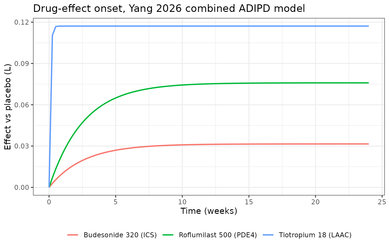
Effect onset over 24 weeks. The anti-inflammatory arms rise over several weeks; the bronchodilator arm is at plateau by the first observation.
# Half of the anti-inflammatory onset is reached at log(2)/0.386 = 1.80 weeks.
ics <- dplyr::filter(s_on, Arm == "Budesonide 320 (ICS)")
half_t <- approx(ics$effect / max(ics$effect), ics$time, xout = 0.5)$y
cat(sprintf("ICS onset half-time: %.3f weeks (expected %.3f)\n",
            half_t, log(2) / exp(ui_adipd$theta[["lonset_ai"]])))
#> ICS onset half-time: 1.796 weeks (expected 1.794)
stopifnot(abs(half_t - log(2) / exp(ui_adipd$theta[["lonset_ai"]])) < 0.05)

# Bronchodilator onset is essentially complete within the first week.
tio <- dplyr::filter(s_on, Arm == "Tiotropium 18 (LAAC)")
stopifnot(tio$effect[tio$time == 1] / max(tio$effect) > 0.99)
Check 8 – background therapy contributes in placebo arms
Background (non-randomized) therapy is present whether or not the arm received a study drug, so it is deliberately not gated on active treatment. A placebo arm in a trial where half the patients stay on inhaled corticosteroids therefore sits above a placebo arm with no background therapy.
ev_bg <- make_events(list(
  adipd_covs(),
  adipd_covs(BGTHER_ICS_RUNIN_PCT = 50, BGTHER_ICS_MAINT_PCT = 50),
  adipd_covs(BGTHER_LAAC_RUNIN_PCT = 50, BGTHER_LAAC_MAINT_PCT = 50)
), times = c(0, 24))
s_bg <- solve_typical(ui_adipd, ev_bg)
#> Warning: No sigma parameters in the model
#> Warning: some etas defaulted to non-mu referenced, possible parsing error: eta_study_isv_cv_bd, eta_study_isv_cv_ai, eta_arm_base, etadps, etaeffref_vil
#> as a work-around try putting the mu-referenced expression on a simple line
#> ℹ omega/sigma items treated as zero: 'eta_study_base', 'eta_study_dps', 'eta_study_pmx', 'eta_study_isv_cv_bd', 'eta_study_isv_cv_ai', 'eta_study_age', 'eta_study_smoke', 'eta_study_bgics', 'eta_study_bglaba', 'eta_study_bglaac', 'eta_arm_base', 'etabase', 'etadps', 'etaeffref_vil', 'etapowSd_FEV1'
#> Warning: multi-subject simulation without without 'omega'
w_bg <- s_bg[s_bg$time == 24, ]

data.frame(
  `Placebo arm` = c("No background therapy", "50% on background ICS",
                    "50% on background LAAC"),
  `FEV1 at week 24 (L)` = w_bg$FEV1,
  check.names = FALSE
) |> knitr::kable(digits = 4)| Placebo arm | FEV1 at week 24 (L) |
|---|---|
| No background therapy | 1.0791 |
| 50% on background ICS | 1.0988 |
| 50% on background LAAC | 1.1377 |
stopifnot(w_bg$FEV1[2] > w_bg$FEV1[1], w_bg$FEV1[3] > w_bg$FEV1[1])Check 9 – post-bronchodilator records
A post-bronchodilator record is predicted from a baseline raised by
the median absolute reversibility of 0.18 L, and sees only
rel_postbd = 0.531 of the long-acting bronchodilator
effect.
ev_pbd <- make_events(list(
  adipd_covs(CONMED_TIOTROPIUM_DOSE = 18),
  adipd_covs(CONMED_TIOTROPIUM_DOSE = 18, MEAS_POSTBD = 1),
  adipd_covs(),
  adipd_covs(MEAS_POSTBD = 1)
), times = c(0, 24))
s_pbd <- solve_typical(ui_adipd, ev_pbd)
#> Warning: No sigma parameters in the model
#> Warning: some etas defaulted to non-mu referenced, possible parsing error: eta_study_isv_cv_bd, eta_study_isv_cv_ai, eta_arm_base, etadps, etaeffref_vil
#> as a work-around try putting the mu-referenced expression on a simple line
#> ℹ omega/sigma items treated as zero: 'eta_study_base', 'eta_study_dps', 'eta_study_pmx', 'eta_study_isv_cv_bd', 'eta_study_isv_cv_ai', 'eta_study_age', 'eta_study_smoke', 'eta_study_bgics', 'eta_study_bglaba', 'eta_study_bglaac', 'eta_arm_base', 'etabase', 'etadps', 'etaeffref_vil', 'etapowSd_FEV1'
#> Warning: multi-subject simulation without without 'omega'
w_pbd <- s_pbd[s_pbd$time == 24, ]

eff_pre  <- w_pbd$FEV1[1] - w_pbd$FEV1[3]
eff_post <- w_pbd$FEV1[2] - w_pbd$FEV1[4]
base_shift <- s_pbd$FEV1[s_pbd$time == 0][4] - s_pbd$FEV1[s_pbd$time == 0][3]

cat(sprintf("Baseline shift for a post-SABD record: %.5f L (0.18 L x the lognormal-mean scaling %.5f)\n",
            base_shift, exp(ui_adipd$theta[["cv_base"]]^2 / 2)))
#> Baseline shift for a post-SABD record: 0.18512 L (0.18 L x the lognormal-mean scaling 1.02847)
cat(sprintf("Tiotropium effect: pre-BD %.4f L, post-BD %.4f L, ratio %.4f (rel_postbd = %.4f)\n",
            eff_pre, eff_post, eff_post / eff_pre, ui_adipd$theta[["rel_postbd"]]))
#> Tiotropium effect: pre-BD 0.1172 L, post-BD 0.0622 L, ratio 0.5310 (rel_postbd = 0.5310)

# The baseline-on-effect multiplier rel_bd is built from the PRE-bronchodilator
# baseline for both record types (source control stream:
# 'RELBD = 1 + RELBDBSLslp * (B - 1.2)', with B the pre-SABD baseline), so the
# post/pre bronchodilator-effect ratio is an EXACT identity equal to
# rel_postbd, not merely a bound. The baseline shift is 0.18 L carried through
# the same log-normal-mean scaling as the baseline itself.
stopifnot(
  abs(base_shift - 0.18 * exp(ui_adipd$theta[["cv_base"]]^2 / 2)) < 1e-12,
  abs(eff_post / eff_pre - ui_adipd$theta[["rel_postbd"]]) < 1e-12
)
Check 10 – a stochastic per-study simulation (paper Figure 4)
Figure 4 of the paper simulates vilanterol 25 ug and vilanterol / fluticasone furoate 25/200 ug over 24 weeks across a virtual population and plots the week-24 FEV1 distribution faceted by sex and treatment, reporting that males show higher FEV1 than females on average and that the two treatments perform only slightly differently.
The combined model carries random effects at three levels and rxode2
draws one level per solve, so this simulation treats one rxode2
id as one study arm – the level at which
eta_arm_base and the eta_study_* effects are
defined. Cohort sizes are kept modest (60 arms per group) as this is an
illustrative reproduction, not a production VPC.
rxode2::rxSetSeed(20260912)
n_arm_sim <- 60L

arms <- expand.grid(
  sex = c("Male", "Female"),
  trt = c("VI 25", "VI/FF 25/200"),
  rep = seq_len(n_arm_sim), stringsAsFactors = FALSE
)
ev_f4 <- make_events(lapply(seq_len(nrow(arms)), function(i) {
  adipd_covs(
    SEXF = if (arms$sex[i] == "Male") 0 else 1,
    DTYPE_AGGREGATED = 1, N_ARM = 200,
    CONMED_VILANTEROL_DOSE = 25,
    CONMED_FLUTICASONEFUROATE_DOSE = if (arms$trt[i] == "VI 25") 0 else 200
  )
}), times = c(0, 24))

sim_f4 <- rxode2::rxSolve(ui_adipd, ev_f4, returnType = "data.frame")
#> ℹ omega/sigma items treated as zero: 'etaeffref_vil'
sim_f4 <- sim_f4[sim_f4$time == 24, ]
sim_f4$sex <- arms$sex[sim_f4$id]
sim_f4$trt <- arms$trt[sim_f4$id]

ggplot(sim_f4, aes(FEV1, colour = sex)) +
  geom_density(linewidth = 0.8) +
  facet_wrap(~ trt) +
  labs(x = "FEV1 at week 24 (L)", y = "Density", colour = NULL,
       title = "Simulated week-24 FEV1 by sex and treatment") +
  theme_bw() + theme(legend.position = "bottom")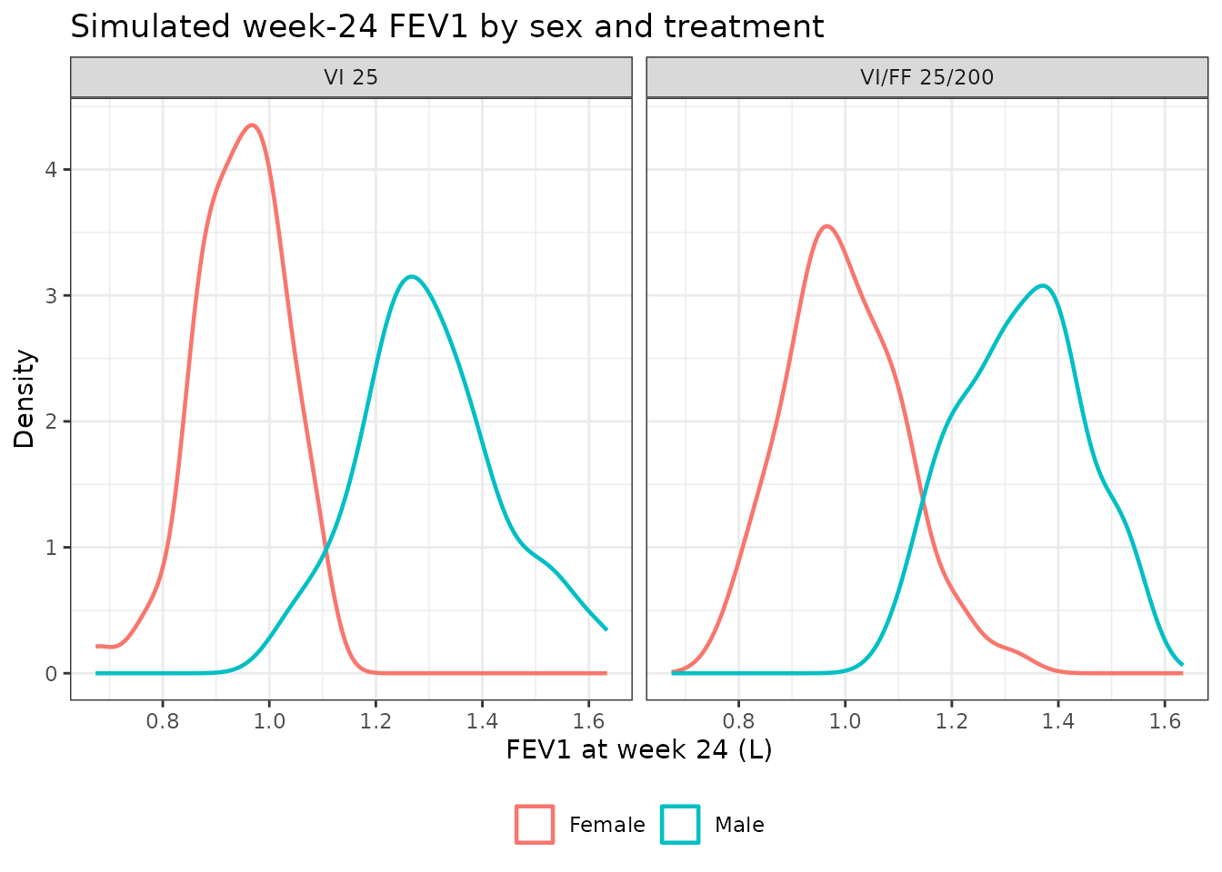
Week-24 FEV1 by sex and treatment, simulated from the combined ADIPD model. Reproduces the structure of Figure 4 of Yang 2026.
f4_tab <- sim_f4 |>
  dplyr::group_by(trt, sex) |>
  dplyr::summarise(mean_FEV1 = mean(FEV1), sd_FEV1 = sd(FEV1), .groups = "drop") |>
  dplyr::rename("Treatment" = trt, "Sex" = sex,
                "Mean FEV1 (L)" = mean_FEV1, "SD across arms (L)" = sd_FEV1)
knitr::kable(f4_tab, digits = 4)| Treatment | Sex | Mean FEV1 (L) | SD across arms (L) |
|---|---|---|---|
| VI 25 | Female | 0.9692 | 0.1175 |
| VI 25 | Male | 1.2888 | 0.1348 |
| VI/FF 25/200 | Female | 1.0279 | 0.1108 |
| VI/FF 25/200 | Male | 1.3084 | 0.1223 |
male_minus_female <- mean(sim_f4$FEV1[sim_f4$sex == "Male"]) -
  mean(sim_f4$FEV1[sim_f4$sex == "Female"])
cat(sprintf("Mean male - female difference: %.4f L\n", male_minus_female))
#> Mean male - female difference: 0.3001 L

# The sex effect is a large, structural, typical-value difference (the
# coefficient implies a female/male baseline ratio of 0.75, i.e. roughly a
# 0.27 L gap at this baseline), so it dominates the cohort noise by a wide
# margin. The bound below is a MAGNITUDE band around that structural value,
# not a bound fitted to one draw: a mis-signed or dropped sex coefficient
# lands outside it, while resampling the cohort moves it by ~0.01 L.
stopifnot(male_minus_female > 0.15, male_minus_female < 0.40)

# Adding fluticasone furoate on top of vilanterol must help, but only slightly
# (the paper describes the two treatments as performing "slightly differently").
trt_gain <- mean(sim_f4$FEV1[sim_f4$trt == "VI/FF 25/200"]) -
  mean(sim_f4$FEV1[sim_f4$trt == "VI 25"])
cat(sprintf("Mean VI/FF - VI difference: %.4f L\n", trt_gain))
#> Mean VI/FF - VI difference: 0.0391 L
stopifnot(trt_gain > 0, trt_gain < 0.10)
Assumptions and deviations
Everything below is a deliberate, documented choice; none changes a published value.
Data-interface re-encoding (both models). The source
data set identifies a study arm’s treatments through up to three
positional slots, each a (drgNoN, avdostotN) pair of an
integer drug code and its average total daily dose, with the regimen and
device carried in parallel dosfreqNoN,
dosfrmNSM and DRGOLN slots. The packaged
models instead read one named CONMED_<drug>_DOSE
column per compound plus named FORM_* selectors. This is
the same information keyed by drug name rather than by slot, it is
mathematically identical, and it matches the
CONMED_<INN>_DOSE convention already used by the
repository’s other multi-drug meta-analyses. Ten of the 23 compounds
carry a constant effect with no dose-response; for those the model keys
on the dose column being non-zero, and the column value carries no
dose-proportionality – the idiom already recorded for
CONMED_MTX_DOSE.
Post-bronchodilator baseline reconciliation
(FEV1_PBD_ANCHOR). For six of the aggregated
studies the source adds DV * (1 - 0.884349) to the
prediction, reconciling an absolute FEV1 that had been reconstructed
from a post-bronchodilator baseline. Using the dependent variable inside
the prediction cannot be expressed in rxode2 and is not meaningful for
forward simulation, so the value is exposed as an explicit input column
that must be zero for simulation. Setting it to zero
reproduces the published model exactly for every record outside those
six studies, and the parameter itself (postbd_recon =
0.884349, Table S3) is retained so the dependence stays visible and
auditable.
Random-effect levels. The source uses NONMEM
$LEVEL with a study super-ID plus an interoccasion-like arm
random effect, needing ten separate N(0,1) etas for the
arm level because $LEVEL cannot nest an arm inside a study;
only one of the ten is ever active for a given record. The packaged
model collapses those to a single eta_arm_base, which is
exact whenever one rxode2 id is one study arm. rxode2 draws
one level of random effects per solve, so a simulation needing both a
study and an arm level must solve once per level or supply the etas
explicitly; the naming (eta_study_* for study level,
eta_arm_base for arm level, unprefixed etas for subject
level) records which is which.
Convention-check warnings.
checkModelConventions() reports no errors on either model
and six parameter_naming warnings on the combined model,
for etas whose name does not resolve to a declared fixed-effect
parameter. Five are the missing-covariate imputation random effects
(eta_study_age, eta_study_smoke,
eta_study_bgics, eta_study_bglaba,
eta_study_bglaac), whose regressions have hardcoded
coefficients in the source control stream and therefore no
ini() parameter to pair with; the sixth is
eta_arm_base, which names a random-effect level (the study
arm) that the checker’s eta_study_ /
eta<param> prefix rules do not yet recognise. The
individual-patient model is convention-clean.
Dead parameters not carried. Three Table S3 rows –
the imputation variances for prior ICS, LABA and LAAC medication
history – feed only the lowest-disease-severity adjustment
THETA(31), which was estimated to zero and whose single
consumer is commented out of the final control stream
(LOWDSact = LOWDS). Two further control-stream thetas fixed
to zero (log.Placebo.T50,
log.P.fast.plac.resp) belong to the placebo mixture that
Section 2.3.1 removed, and THETA(31) itself likewise has no
surviving equation. None appears in any prediction, so none is encoded;
the three severity-covariate thetas that the source does keep
as live-but-fixed-to-zero structure (e_gold_lo_base,
e_gold_hi_base, e_gold_dps) are retained so a
user can un-fix them.
Missing-value sentinels. The imputation branches are
reached through the source’s in-band sentinels, preserved here:
-99 for a missing age, smoking fraction or GOLD stage, and
9999 (class not used, treated as zero) or 7777
(class used, fraction unreported) for the background-therapy columns. A
complete data set never reaches them.
Sex coding. The source codes sex as
SEX = 1 for male, centred at the pooled male fraction
0.671. The canonical column is SEXF (1 = female), so the
identical algebra is written as (0.329 - SEXF) with the
published coefficient and sign unchanged. The resulting female/male
baseline ratio of 0.747 agrees with the 0.752 implied by the
individual-patient model’s own coefficient and with the paper’s repeated
statement that female sex relates to a lower baseline.
Erratum search. No erratum or corrigendum for doi:10.1002/psp4.70059 was found on the publisher’s page or in the EuropePMC record as of 2026-09-12.
Upstream source. The structural skeleton and the entire aggregated data set are inherited from Llanos-Paez 2023 (J Pharmacokinet Pharmacodyn 50:297-314). Every parameter value encoded here is re-estimated and reported in Yang 2026’s own Table S2 / Table S3, so no value is taken from the upstream paper; only the narrative attribution of the structure is.
A note on Table S3’s fluticasone row. Table S3
displays THETA(38) as “Relative reference efficacy of
fluticasone 200 ug q.d. compared to b.i.d = 0.04”. The control stream
shows that theta used as
TVDMX32QD = THETA(38)/REFDFF*(ED5032QD+REFDFF) with
REFDFF = 100, i.e. it is the fluticasone
furoate (drug 32) reference efficacy at 100 ug/day, not a ratio
involving fluticasone propionate (drug 9). The model follows the control
stream. This is also why the two molecules carry separate covariate
columns.