Glycochenodeoxycholic acid 3-O-sulfate, an OATP1B3 / OAT3 biomarker (Ujihira 2025)
Source:vignettes/articles/Ujihira_2025_glycochenodeoxycholicAcidSulfate.Rmd
Ujihira_2025_glycochenodeoxycholicAcidSulfate.RmdModel and source
- Citation: Ujihira Y, Georgiev V, Ogungbenro K, Galetin A. Population Pharmacokinetic Modeling of Glycochenodeoxycholic Acid 3-O-Sulfate (GCDCA-S) as Endogenous Biomarker of OATP1B3 and OAT3 Transporters. Clin Pharmacol Ther. 2025;118(6):1532-1542. doi:10.1002/cpt.70023. Structural equations from Eqs 1-4 of the main text; all parameter values from Table 2. Supplementary Material S1 (Tables S1-S7) was also used. The unbound fractions that convert each perpetrator’s modelled total plasma concentration to the unbound concentration driving inhibition are reported nowhere in the paper or its supplement; they are taken from the two upstream models the paper adopts – rifampicin fu = 0.11 (Barnett 2018 Clin Pharmacol Ther 104:564-574 Table 1 footnote c) and probenecid fu = 0.062 (Ahmad 2021 CPT Pharmacometrics Syst Pharmacol 10:467-477) – and each is pinned by a published answer key: the Table S4 AUCR of 13 at 600 mg rifampicin and the Table S4 renal-clearance ratio of 0.1 under 500 mg QID probenecid. See the vignette Errata.
- Article: https://doi.org/10.1002/cpt.70023
Glycochenodeoxycholic acid 3-O-sulfate (GCDCA-S) is a sulfated bile-acid conjugate proposed by the International Transporter Consortium as a Tier 2 endogenous biomarker of hepatic OATP1B3 and renal OAT3. Ujihira 2025 is the first mechanistic population-PK model for it, and it quantifies two things that were previously unknown: the biomarker’s zero-order synthesis rate, and the split between its hepatobiliary and renal elimination routes.
The distinctive feature of this extraction is that the model is a
single coupled three-drug system. The paper fit the
GCDCA-S turnover model simultaneously with the perpetrator PK of
rifampicin and probenecid (Figure 2), and the two inhibition constants
plus the probenecid fold-change X are joint estimates
across that system. The model file therefore carries all five ODE states
in one place, so a user can dose a perpetrator and read the biomarker
response directly, without a two-step simulate-then-feed workflow.
mod <- rxode2::rxode(readModelDb("Ujihira_2025_glycochenodeoxycholicAcidSulfate"))
#> ℹ parameter labels from comments will be replaced by 'label()'
mod
#>  ── rxode2-based free-form 5-cmt ODE model ──────────────────────────────────────
#>  ── Initalization: ──
#> Fixed Effects ($theta):
#>          lksyn            lvc      lcl_renal     lcl_nonren      ltlag_rif
#>     0.00000000     1.56861592    -1.17118298     2.70805020    -0.57981850
#>        ld1_rif        lvc_rif        lcl_rif   lkiu_oatp1b3         fu_rif
#>    -0.17435339     3.55534806     1.90210753    -4.71053070     0.11000000
#>       lka_prob       lvc_prob       lcl_prob      lkiu_oat3        fu_prob
#>     0.09531018     2.83321334    -0.05129329     0.99325177     0.06200000
#>     e_prob_clh         propSd propSd_Ugcdcas     propSd_rif      addSd_rif
#>    -0.41176470     0.45000000     0.29000000     0.20000000     0.20000000
#>    propSd_prob     addSd_prob
#>     0.23000000     0.00100000
#>
#> Omega ($omega):
#>               etalksyn etalcl_renal etaltlag_rif etald1_rif etalcl_rif
#> etalksyn     0.3163576    0.0000000    0.0000000  0.0000000  0.0000000
#> etalcl_renal 0.0000000    0.0560025    0.0000000  0.0000000  0.0000000
#> etaltlag_rif 0.0000000    0.0000000    0.1919877  0.0000000  0.0000000
#> etald1_rif   0.0000000    0.0000000    0.0000000  0.4656585  0.0000000
#> etalcl_rif   0.0000000    0.0000000    0.0000000  0.0000000  0.0318856
#> etalvc_prob  0.0000000    0.0000000    0.0000000  0.0000000  0.0000000
#> etalcl_prob  0.0000000    0.0000000    0.0000000  0.0000000  0.0000000
#> etalkiu_oat3 0.0000000    0.0000000    0.0000000  0.0000000  0.0000000
#>              etalvc_prob etalcl_prob etalkiu_oat3
#> etalksyn       0.0000000   0.0000000    0.0000000
#> etalcl_renal   0.0000000   0.0000000    0.0000000
#> etaltlag_rif   0.0000000   0.0000000    0.0000000
#> etald1_rif     0.0000000   0.0000000    0.0000000
#> etalcl_rif     0.0000000   0.0000000    0.0000000
#> etalvc_prob    0.0917476   0.0000000    0.0000000
#> etalcl_prob    0.0000000   0.0703679    0.0000000
#> etalkiu_oat3   0.0000000   0.0000000    0.0974856
#> attr(,"lotriLabels")
#> [1] "Table 2, GCDCA-S IIV ksyn = 61% (RSE 15%); log(1 + 0.61^2)"
#> [2] "Table 2, GCDCA-S IIV CLR  = 24% (RSE 25%); log(1 + 0.24^2)"
#> [3] "Table 2, RIF IIV Tlag     = 46% (RSE 32%); log(1 + 0.46^2)"
#> [4] "Table 2, RIF IIV Tk0      = 77% (RSE 37%); log(1 + 0.77^2)"
#> [5] "Table 2, RIF IIV CL       = 18% (RSE 35%); log(1 + 0.18^2)"
#> [6] "Table 2, PROB IIV V       = 31% (RSE 28%); log(1 + 0.31^2)"
#> [7] "Table 2, PROB IIV CL      = 27% (RSE 20%); log(1 + 0.27^2)"
#> [8] "Table 2, PROB IIV Ki,u,OAT3 = 32% (RSE 27%); log(1 + 0.32^2)"
#> attr(,"lotriFix")
#>              etalksyn etalcl_renal etaltlag_rif etald1_rif etalcl_rif
#> etalksyn        FALSE        FALSE        FALSE      FALSE      FALSE
#> etalcl_renal    FALSE        FALSE        FALSE      FALSE      FALSE
#> etaltlag_rif    FALSE        FALSE        FALSE      FALSE      FALSE
#> etald1_rif      FALSE        FALSE        FALSE      FALSE      FALSE
#> etalcl_rif      FALSE        FALSE        FALSE      FALSE      FALSE
#> etalvc_prob     FALSE        FALSE        FALSE      FALSE      FALSE
#> etalcl_prob     FALSE        FALSE        FALSE      FALSE      FALSE
#> etalkiu_oat3    FALSE        FALSE        FALSE      FALSE      FALSE
#>              etalvc_prob etalcl_prob etalkiu_oat3
#> etalksyn           FALSE       FALSE        FALSE
#> etalcl_renal       FALSE       FALSE        FALSE
#> etaltlag_rif       FALSE       FALSE        FALSE
#> etald1_rif         FALSE       FALSE        FALSE
#> etalcl_rif         FALSE       FALSE        FALSE
#> etalvc_prob        FALSE       FALSE        FALSE
#> etalcl_prob        FALSE       FALSE        FALSE
#> etalkiu_oat3       FALSE       FALSE        FALSE
#>
#> States ($state or $stateDf):
#>   Compartment Number Compartment Name
#> 1                  1          central
#> 2                  2            urine
#> 3                  3      central_rif
#> 4                  4       depot_prob
#> 5                  5     central_prob
#>  ── Multiple Endpoint Model ($multipleEndpoint): ──
#>      variable                    cmt                    dvid*
#> 1      Cc ~ …      cmt='Cc' or cmt=6      dvid='Cc' or dvid=1
#> 2 Ugcdcas ~ … cmt='Ugcdcas' or cmt=7 dvid='Ugcdcas' or dvid=2
#> 3  Cc_rif ~ …  cmt='Cc_rif' or cmt=8  dvid='Cc_rif' or dvid=3
#> 4 Cc_prob ~ … cmt='Cc_prob' or cmt=9 dvid='Cc_prob' or dvid=4
#>   * If dvids are outside this range, all dvids are re-numered sequentially, ie 1,7, 10 becomes 1,2,3 etc
#>
#>  ── μ-referencing ($muRefTable): ──
#>       theta          eta level
#> 1     lksyn     etalksyn    id
#> 2 lcl_renal etalcl_renal    id
#> 3 ltlag_rif etaltlag_rif    id
#> 4   ld1_rif   etald1_rif    id
#> 5   lcl_rif   etalcl_rif    id
#> 6  lvc_prob  etalvc_prob    id
#> 7  lcl_prob  etalcl_prob    id
#> 8 lkiu_oat3 etalkiu_oat3    id
#>
#>  ── Model (Normalized Syntax): ──
#> function() {
#>     compartmentData <- list(central = list(analyte = "glycochenodeoxycholic acid 3-O-sulfate",
#>         units = "umol", specimen = "plasma", verified = TRUE),
#>         urine = list(analyte = "glycochenodeoxycholic acid 3-O-sulfate",
#>             units = "umol", specimen = "urine", verified = TRUE),
#>         central_rif = list(analyte = "rifampicin", units = "umol",
#>             specimen = "plasma", verified = TRUE), depot_prob = list(analyte = "probenecid",
#>             units = "umol", specimen = "administration site",
#>             verified = TRUE), central_prob = list(analyte = "probenecid",
#>             units = "umol", specimen = "plasma", verified = TRUE))
#>     covariateData <- list(CONMED_PROBENECID = list(description = "Concomitant probenecid co-administration indicator (1 = subject is within a probenecid dosing period; 0 = no probenecid). Gates the concentration-independent fold reduction X in GCDCA-S hepatobiliary clearance that Ujihira 2025 estimated for probenecid's weak OATP1B3 inhibition.",
#>         units = "(binary)", type = "binary", reference_category = "0 (no probenecid co-administration)",
#>         notes = "Time-varying within subject. Probenecid regimen in the source studies (Ujihira 2025 Table 1, studies #2 and #3, adopted from Willemin et al. 2021): 500 mg orally at 6 pm and 11 pm on day 0, then 500 mg at 7 am, 1 pm, 6 pm and 11 pm on days 1 to 7; GCDCA-S plasma and urine sampling begins on day 1. The indicator modifies ONLY the hepatobiliary clearance arm cl_nonren, via the multiplicative factor (1 + e_prob_clh * CONMED_PROBENECID) = 1 / X. It deliberately does NOT gate the renal-clearance inhibition, which is concentration-driven through the probenecid PK model and Ki,u,OAT3 and therefore switches itself off whenever probenecid is not dosed. Set to 1 from the first probenecid dose through the end of the probenecid-phase sampling window; the paper reports no lag or washout term. Rifampicin needs no equivalent indicator because its only effect is the concentration-driven OATP1B3 term."))
#>     covariatesDataExcluded <- list(SEXF = list(description = "Female sex indicator (1 = female, 0 = male).",
#>         units = "(binary)", type = "binary", notes = "Tested on the GCDCA-S synthesis rate ksyn as ksyn,sex = ksyn,male * (1 - SEX * COVSEX) (Supplementary Material S1 Eq. 2, with SEX = 1 for women). The estimate COVSEX = 0.065 carried an RSE of 404% and moved the objective function by only 3 points (OFV -642 -> -639, p > 0.9; Table S3), so sex was excluded from the final model despite the paper's observation that baseline GCDCA-S is higher in men."))
#>     description <- "Coupled three-drug turnover model for the endogenous OATP1B3 / OAT3 biomarker glycochenodeoxycholic acid 3-O-sulfate (GCDCA-S) in healthy adults (Ujihira 2025), fit simultaneously with the perpetrator PK of rifampicin and probenecid. GCDCA-S is produced at a zero-order synthesis rate ksyn and eliminated by hepatobiliary clearance CLh (the dominant route, ~98% of total systemic clearance, giving fe < 5%) and renal clearance CLR, with plasma concentration and cumulative urinary amount as the two biomarker outputs. Rifampicin competitively inhibits CLh through the unbound OATP1B3 constant Ki,u,OATP1B3 driven by its own one-compartment zero-order-absorption PK; probenecid competitively inhibits CLR through the unbound OAT3 constant Ki,u,OAT3 driven by its own one-compartment first-order-absorption PK, and additionally reduces CLh by a concentration-independent 1.7-fold factor X gated by the binary CONMED_PROBENECID indicator. All three drugs live in this one file because the paper fit them as a single coupled system (Figure 2); dosing rifampicin or probenecid alone drives the corresponding interaction, and dosing neither collapses the model to the inhibitor-free steady-state baseline of about 65 nmol/L (typical value). Perpetrator doses are given in umol, not mg, because the whole system runs in umol / umol per L."
#>     population <- list(species = "human", n_subjects = 24L, n_studies = 3L,
#>         age_range = "20-71 years across the three model-development studies (study #1 50-71; study #2 48-58; study #3 20-55).",
#>         weight_range = "(not extracted; Ujihira 2025 Table 1 does not tabulate body weight, and no allometric or weight covariate appears in the final model.)",
#>         sex_female_pct = 37.5, race_ethnicity = "White in all three model-development studies (Ujihira 2025 Table 1).",
#>         disease_state = "Healthy volunteers. GCDCA-S was monitored as an endogenous biomarker of hepatic OATP1B3 and renal OAT3 activity during transporter drug-drug-interaction studies.",
#>         dose_range = "Endogenous biomarker (no exogenous GCDCA-S dose). Perpetrators: rifampicin single 600 mg oral dose (study #1); probenecid 500 mg orally four times daily (QID) on days 1 to 7, preceded by two loading doses on day 0 (studies #2 and #3).",
#>         regions = "(not extracted; Ujihira 2025 Table 1 reports ethnicity but not study region for the three development studies.)",
#>         notes = "Pooled from three healthy-volunteer crossover studies, each with a control occasion and an inhibitor occasion: study #1 Tatosian et al. 2021 (n = 6; 3 male, 3 female; microdose probe cocktail +/- rifampicin), study #2 Willemin et al. 2021 (n = 6; 6 female; +/- probenecid), study #3 unpublished data of the same design as study #2 (n = 12; 12 male). Sex percentage is 9 female of 24. 430 GCDCA-S plasma samples and 175 GCDCA-S urine samples were fit simultaneously with 153 perpetrator plasma samples in Monolix 2024R2. Observed GCDCA-S plasma baseline was approximately 80 nmol/L with high between-subject (CV 34-69%) and within-subject diurnal (CV 34-43%) variability. Neither a diurnal-fluctuation function (six forms tested, Table S2) nor a sex effect on ksyn (Table S3) improved the fit, so neither is in the final model. The model was verified against four independent studies (Table S1) not used in fitting.")
#>     reference <- "Ujihira Y, Georgiev V, Ogungbenro K, Galetin A. Population Pharmacokinetic Modeling of Glycochenodeoxycholic Acid 3-O-Sulfate (GCDCA-S) as Endogenous Biomarker of OATP1B3 and OAT3 Transporters. Clin Pharmacol Ther. 2025;118(6):1532-1542. doi:10.1002/cpt.70023. Structural equations from Eqs 1-4 of the main text; all parameter values from Table 2. Supplementary Material S1 (Tables S1-S7) was also used. The unbound fractions that convert each perpetrator's modelled total plasma concentration to the unbound concentration driving inhibition are reported nowhere in the paper or its supplement; they are taken from the two upstream models the paper adopts -- rifampicin fu = 0.11 (Barnett 2018 Clin Pharmacol Ther 104:564-574 Table 1 footnote c) and probenecid fu = 0.062 (Ahmad 2021 CPT Pharmacometrics Syst Pharmacol 10:467-477) -- and each is pinned by a published answer key: the Table S4 AUCR of 13 at 600 mg rifampicin and the Table S4 renal-clearance ratio of 0.1 under 500 mg QID probenecid. See the vignette Errata."
#>     units <- list(time = "h", dosing = "umol", concentration = "umol/L")
#>     vignette <- "Ujihira_2025_glycochenodeoxycholicAcidSulfate"
#>     ini({
#>         lksyn <- 0
#>         label("GCDCA-S zero-order synthesis rate ksyn (umol/h)")
#>         lvc <- fix(1.56861591791385)
#>         label("GCDCA-S volume of distribution Vc (L)")
#>         lcl_renal <- -1.17118298150295
#>         label("GCDCA-S renal clearance CLR (L/h)")
#>         lcl_nonren <- 2.70805020110221
#>         label("GCDCA-S hepatobiliary clearance CLh (L/h)")
#>         ltlag_rif <- -0.579818495252942
#>         label("Rifampicin absorption lag time Tlag,RIF (h)")
#>         ld1_rif <- -0.174353387144778
#>         label("Rifampicin zero-order absorption duration Tk0,RIF (h)")
#>         lvc_rif <- 3.55534806148941
#>         label("Rifampicin volume of distribution V,RIF (L)")
#>         lcl_rif <- 1.90210752639692
#>         label("Rifampicin clearance CL,RIF (L/h)")
#>         lkiu_oatp1b3 <- -4.71053070164592
#>         label("Rifampicin unbound OATP1B3 inhibition constant Ki,u,OATP1B3 (umol/L)")
#>         fu_rif <- fix(0.11)
#>         label("Rifampicin fraction unbound in plasma (unitless)")
#>         lka_prob <- 0.0953101798043249
#>         label("Probenecid absorption rate constant ka,PROB (1/h)")
#>         lvc_prob <- 2.83321334405622
#>         label("Probenecid volume of distribution V,PROB (L)")
#>         lcl_prob <- -0.0512932943875506
#>         label("Probenecid clearance CL,PROB (L/h)")
#>         lkiu_oat3 <- 0.993251773010283
#>         label("Probenecid unbound OAT3 inhibition constant Ki,u,OAT3 (umol/L)")
#>         fu_prob <- fix(0.062)
#>         label("Probenecid fraction unbound in plasma (unitless)")
#>         e_prob_clh <- -0.4117647
#>         label("Multiplicative change in GCDCA-S hepatobiliary clearance during probenecid co-administration (unitless)")
#>         propSd <- c(0, 0.45)
#>         label("Proportional residual error, GCDCA-S plasma (fraction)")
#>         propSd_Ugcdcas <- c(0, 0.29)
#>         label("Proportional residual error, GCDCA-S urine (fraction)")
#>         propSd_rif <- c(0, 0.2)
#>         label("Proportional residual error, rifampicin plasma (fraction)")
#>         addSd_rif <- fix(0, 0.2)
#>         label("Additive residual error, rifampicin plasma (umol/L)")
#>         propSd_prob <- c(0, 0.23)
#>         label("Proportional residual error, probenecid plasma (fraction)")
#>         addSd_prob <- fix(0, 0.001)
#>         label("Additive residual error, probenecid plasma (umol/L)")
#>         etalksyn ~ 0.3163576
#>         label("Table 2, GCDCA-S IIV ksyn = 61% (RSE 15%); log(1 + 0.61^2)")
#>         etalcl_renal ~ 0.0560025
#>         label("Table 2, GCDCA-S IIV CLR  = 24% (RSE 25%); log(1 + 0.24^2)")
#>         etaltlag_rif ~ 0.1919877
#>         label("Table 2, RIF IIV Tlag     = 46% (RSE 32%); log(1 + 0.46^2)")
#>         etald1_rif ~ 0.4656585
#>         label("Table 2, RIF IIV Tk0      = 77% (RSE 37%); log(1 + 0.77^2)")
#>         etalcl_rif ~ 0.0318856
#>         label("Table 2, RIF IIV CL       = 18% (RSE 35%); log(1 + 0.18^2)")
#>         etalvc_prob ~ 0.0917476
#>         label("Table 2, PROB IIV V       = 31% (RSE 28%); log(1 + 0.31^2)")
#>         etalcl_prob ~ 0.0703679
#>         label("Table 2, PROB IIV CL      = 27% (RSE 20%); log(1 + 0.27^2)")
#>         etalkiu_oat3 ~ 0.0974856
#>         label("Table 2, PROB IIV Ki,u,OAT3 = 32% (RSE 27%); log(1 + 0.32^2)")
#>     })
#>     model({
#>         ksyn <- exp(lksyn + etalksyn)
#>         vc <- exp(lvc)
#>         cl_renal <- exp(lcl_renal + etalcl_renal)
#>         cl_nonren <- exp(lcl_nonren)
#>         tlag_rif <- exp(ltlag_rif + etaltlag_rif)
#>         d1_rif <- exp(ld1_rif + etald1_rif)
#>         vc_rif <- exp(lvc_rif)
#>         cl_rif <- exp(lcl_rif + etalcl_rif)
#>         kiu_oatp1b3 <- exp(lkiu_oatp1b3)
#>         ka_prob <- exp(lka_prob)
#>         vc_prob <- exp(lvc_prob + etalvc_prob)
#>         cl_prob <- exp(lcl_prob + etalcl_prob)
#>         kiu_oat3 <- exp(lkiu_oat3 + etalkiu_oat3)
#>         dur(central_rif) <- d1_rif
#>         alag(central_rif) <- tlag_rif
#>         Cc_rif <- central_rif/vc_rif
#>         Cc_prob <- central_prob/vc_prob
#>         cu_rif <- fu_rif * Cc_rif
#>         cu_prob <- fu_prob * Cc_prob
#>         cl_nonren_eff <- cl_nonren/(1 + cu_rif/kiu_oatp1b3) *
#>             (1 + e_prob_clh * CONMED_PROBENECID)
#>         cl_renal_eff <- cl_renal/(1 + cu_prob/kiu_oat3)
#>         Cc <- central/vc
#>         d/dt(central) <- ksyn - (cl_nonren_eff + cl_renal_eff) *
#>             Cc
#>         d/dt(urine) <- cl_renal_eff * Cc
#>         d/dt(central_rif) <- -cl_rif/vc_rif * central_rif
#>         d/dt(depot_prob) <- -ka_prob * depot_prob
#>         d/dt(central_prob) <- ka_prob * depot_prob - cl_prob/vc_prob *
#>             central_prob
#>         central(0) <- ksyn/(cl_nonren + cl_renal) * vc
#>         urine(0) <- 0
#>         Ugcdcas <- urine
#>         Cc ~ prop(propSd)
#>         Ugcdcas ~ prop(propSd_Ugcdcas)
#>         Cc_rif ~ add(addSd_rif) + prop(propSd_rif)
#>         Cc_prob ~ add(addSd_prob) + prop(propSd_prob)
#>     })
#> }
The model declares four endpoints, so rxode2 places their slots
after the five ODE states. Observation records in every event
table below therefore use cmt = "Cc" and not
cmt = "central": with more than one declared endpoint,
cmt = "central" is rejected with
'dvid'->'cmt' or 'cmt' on observation record. Because
Cc already has an endpoint slot from the model definition,
naming it on an observation row injects nothing and renumbers nothing,
and rxSolve() returns every model variable as an output
column regardless of which endpoint is named.
mod$predDf[, c("var", "cond", "cmt", "dvid")]
#>       var    cond cmt dvid
#> 1      Cc      Cc   6    1
#> 2 Ugcdcas Ugcdcas   7    2
#> 3  Cc_rif  Cc_rif   8    3
#> 4 Cc_prob Cc_prob   9    4
mod$state
#> [1] "central"      "urine"        "central_rif"  "depot_prob"   "central_prob"
Population and biological context
pop <- readModelDb("Ujihira_2025_glycochenodeoxycholicAcidSulfate")()$population
str(pop, max.level = 1)
#> List of 11
#>  $ species       : chr "human"
#>  $ n_subjects    : int 24
#>  $ n_studies     : int 3
#>  $ age_range     : chr "20-71 years across the three model-development studies (study #1 50-71; study #2 48-58; study #3 20-55)."
#>  $ weight_range  : chr "(not extracted; Ujihira 2025 Table 1 does not tabulate body weight, and no allometric or weight covariate appea"| __truncated__
#>  $ sex_female_pct: num 37.5
#>  $ race_ethnicity: chr "White in all three model-development studies (Ujihira 2025 Table 1)."
#>  $ disease_state : chr "Healthy volunteers. GCDCA-S was monitored as an endogenous biomarker of hepatic OATP1B3 and renal OAT3 activity"| __truncated__
#>  $ dose_range    : chr "Endogenous biomarker (no exogenous GCDCA-S dose). Perpetrators: rifampicin single 600 mg oral dose (study #1); "| __truncated__
#>  $ regions       : chr "(not extracted; Ujihira 2025 Table 1 reports ethnicity but not study region for the three development studies.)"
#>  $ notes         : chr "Pooled from three healthy-volunteer crossover studies, each with a control occasion and an inhibitor occasion: "| __truncated__
The model was developed on 24 healthy White volunteers pooled from three crossover studies, each with a control occasion and an inhibitor occasion (Ujihira 2025 Table 1): Tatosian et al. 2021 (n = 6, 3 male / 3 female, single 600 mg oral rifampicin), Willemin et al. 2021 (n = 6, all female, probenecid 500 mg four times daily on days 1-7 after two day-0 loading doses), and an unpublished study of the same design as Willemin (n = 12, all male). 430 GCDCA-S plasma samples and 175 GCDCA-S urine samples were fit simultaneously with 153 perpetrator plasma samples in Monolix 2024R2.
Observed GCDCA-S plasma baseline was approximately 80 nmol/L, with high between-subject variability (CV 34-69% across the three studies) and comparable within-subject diurnal variability (CV 34-43%) – both larger than for the Tier 1 biomarker coproporphyrin I. Six diurnal-fluctuation functions (Table S2) and a sex effect on the synthesis rate (Table S3) were each tested and each failed to improve the fit, so neither appears in the final model.
Source trace
Every structural equation and every ini() value, with
its location in the source.
| Model element | Value | Source location |
|---|---|---|
| Plasma turnover ODE, no inhibitor | dC/dt = [ksyn - (C*CLh + C*CLR)] / Vc |
Eq. 1, main text p. 1535 |
| Plasma turnover ODE, with inhibitors | dC/dt = [ksyn - (C*CLh/(1+Cu_RIF/Ki_u_OATP1B3)*(1/X) + C*CLR/(1+Cu_PROB/Ki_u_OAT3))] / Vc |
Eq. 2, main text p. 1535 |
| Urine ODE, no inhibitor | dA/dt = C*CLR |
Eq. 3, main text p. 1535 |
| Urine ODE, with probenecid | dA/dt = C*CLR/(1+Cu_PROB/Ki_u_OAT3) |
Eq. 4, main text p. 1535 |
| Rifampicin structure | 1-compartment, zero-order absorption after a lag, linear elimination | Methods “Structural models”; Figure 2 left panel |
| Probenecid structure | 1-compartment, first-order absorption, linear elimination | Methods “Structural models”; Figure 2 right panel |
lksyn = log(1.0) umol/h |
1.0 (RSE 18%) | Table 2, GCDCA-S k syn
|
lvc = fixed(log(4.8)) L |
4.8 (FIXED) | Table 2, GCDCA-S V c,GCDCA-S
|
lcl_renal = log(0.31) L/h |
0.31 (RSE 8%) | Table 2, GCDCA-S CL R,GCDCA-S
|
lcl_nonren = log(15) L/h |
15 (RSE 13%) | Table 2, GCDCA-S CL h,GCDCA-S
|
ltlag_rif = log(0.56) h |
0.56 (RSE 20%) | Table 2, RIF Tlag RIF
|
ld1_rif = log(0.84) h |
0.84 (RSE 41%) | Table 2, RIF Tk0 RIF
|
lvc_rif = log(35) L |
35 (RSE 5%) | Table 2, RIF V RIF
|
lcl_rif = log(6.7) L/h |
6.7 (RSE 8%) | Table 2, RIF CL RIF
|
lkiu_oatp1b3 = log(0.009) umol/L |
0.009 (RSE 29%) | Table 2, RIF K i,unbound,OATP1B3
|
lka_prob = log(1.1) 1/h |
1.1 (RSE 37%) | Table 2, PROB ka PROB
|
lvc_prob = log(17) L |
17 (RSE 10%) | Table 2, PROB V PROB
|
lcl_prob = log(0.95) L/h |
0.95 (RSE 7%) | Table 2, PROB CL PROB
|
lkiu_oat3 = log(2.7) umol/L |
2.7 (RSE 12%) | Table 2, PROB K i,unbound,OAT3
|
e_prob_clh = -0.4118 |
X = 1.7 (RSE 5%), encoded as 1/X - 1 |
Table 2, PROB X; Eq. 2 |
etalksyn = 0.3164 |
IIV 61% (RSE 15%), log(1 + 0.61^2) | Table 2, GCDCA-S IIV |
etalcl_renal = 0.0560 |
IIV 24% (RSE 25%) | Table 2, GCDCA-S IIV |
etaltlag_rif = 0.1920 |
IIV 46% (RSE 32%) | Table 2, RIF IIV |
etald1_rif = 0.4657 |
IIV 77% (RSE 37%) | Table 2, RIF IIV |
etalcl_rif = 0.0319 |
IIV 18% (RSE 35%) | Table 2, RIF IIV |
etalvc_prob = 0.0917 |
IIV 31% (RSE 28%) | Table 2, PROB IIV |
etalcl_prob = 0.0704 |
IIV 27% (RSE 20%) | Table 2, PROB IIV |
etalkiu_oat3 = 0.0975 |
IIV 32% (RSE 27%) | Table 2, PROB IIV |
propSd = 0.45 |
45% (RSE 3%) | Table 2, sigma prop - GCDCA-S plasma
|
propSd_Ugcdcas = 0.29 |
29% (RSE 1%) | Table 2, sigma prop - GCDCA-S urine
|
propSd_rif = 0.20 |
20% (RSE 14%) | Table 2, sigma prop - RIF
|
addSd_rif = fixed(0.2) umol/L |
0.2 (FIXED) | Table 2, sigma add - RIF
|
propSd_prob = 0.23 |
23% (RSE 8%) | Table 2, sigma prop - PROB
|
addSd_prob = fixed(0.001) umol/L |
0.001 (FIXED) | Table 2, sigma add - PROB
|
fu_rif = fixed(0.11) |
not in Ujihira 2025 – see Errata | Barnett 2018 Table 1 footnote c |
fu_prob = fixed(0.062) |
not in Ujihira 2025 – see Errata | Ahmad 2021 Table 1 footnote |
Units of every ODE term (dimensional analysis)
The whole system runs in umol and umol/L (=
uM), which is why perpetrator doses must be supplied in
umol rather than mg.
| Term | Units | Check |
|---|---|---|
central, urine
|
umol | state = amount |
Cc = central / vc |
umol / L = uM | matches the paper’s C_GCDCA-S (uM) |
ksyn |
umol/h | matches the paper’s k syn (umol/h) |
cl_nonren, cl_renal
|
L/h | matches CLh, CLR (L/h) |
(cl_nonren_eff + cl_renal_eff) * Cc |
L/h * umol/L = umol/h | balances d/dt(central)
|
d/dt(urine) = cl_renal_eff * Cc |
umol/h | matches the paper’s A_GCDCA-S (umol) |
cu_rif / kiu_oatp1b3 |
uM / uM = unitless | inhibition term is dimensionless |
e_prob_clh |
unitless | multiplicative factor on cl_nonren
|
central_rif / vc_rif |
umol / L = uM | matches Cu,RIF scale after fu_rif
|
The paper writes Eq. 1 in terms of concentration with the whole
bracket divided by Vc; the file uses the algebraically
identical amount form (d/dt(central) = ksyn - CL*Cc with
Cc = central/vc), which is the standard rxode2 idiom and
makes the urine state directly comparable to the paper’s
A_GCDCA-S in umol.
# Molecular weights used only to convert the published mg doses into the umol
# the model consumes. Rifampicin 822.94 g/mol and probenecid 285.34 g/mol are
# the values already carried by the nlmixr2lib covariate / model registers
# (PubChem CID 135398735 and 4911 agree to 4 significant figures).
MW_RIF  <- 822.94
MW_PROB <- 285.34

dose_umol <- function(mg, mw) mg / mw * 1000

# Typical-value (deterministic) model for the structural checks.
mod0 <- rxode2::zeroRe(mod)

# Analytic baseline from Eq. 1 with dC/dt = 0: Css = ksyn / (CLh + CLR).
ksyn <- 1.0; clh <- 15; clr <- 0.31; vc <- 4.8
css_analytic <- ksyn / (clh + clr)
c(css_umol_per_L = css_analytic, css_nmol_per_L = css_analytic * 1000)
#> css_umol_per_L css_nmol_per_L
#>     0.06531679    65.31678641
Steady-state check
With no perpetrator on board the model must sit at the analytic
baseline ksyn / (CLh + CLR) indefinitely.
ev_ss <- rxode2::et(seq(0, 168, by = 0.5), cmt = "Cc") |> as.data.frame()
ev_ss$CONMED_PROBENECID <- 0

ss <- rxode2::rxSolve(mod0, ev_ss, returnType = "data.frame")
#> ℹ omega/sigma items treated as zero: 'etalksyn', 'etalcl_renal', 'etaltlag_rif', 'etald1_rif', 'etalcl_rif', 'etalvc_prob', 'etalcl_prob', 'etalkiu_oat3'

max_drift <- max(abs(ss$Cc - css_analytic))
c(analytic = css_analytic, simulated = ss$Cc[1], max_abs_drift = max_drift)
#>      analytic     simulated max_abs_drift
#>    0.06531679    0.06531679    0.00000000

stopifnot(max_drift < 1e-10)
The simulated baseline holds at 0.0653168 umol/L (65.32 nmol/L) over 7 days with no drift.
Perturbation-recovery
The model-body initial condition
central(0) <- ksyn/(CLh + CLR) * vc overrides
rxSolve(inits = ), so the state is displaced with events
instead: a bolus dose that doubles the central amount, and an
evid = 6 multiply event that halves it. Both must return to
the same attractor.
c0 <- css_analytic * vc

perturb <- function(ev, label) {
  ev <- as.data.frame(ev)
  ev$CONMED_PROBENECID <- 0
  out <- rxode2::rxSolve(mod0, ev, returnType = "data.frame")
  out$arm <- label
  out
}

up <- perturb(
  rxode2::et(amt = c0, cmt = "central", time = 0) |>
    rxode2::et(seq(0, 6, by = 0.02), cmt = "Cc"),
  "2x baseline (bolus)"
)
#> ℹ omega/sigma items treated as zero: 'etalksyn', 'etalcl_renal', 'etaltlag_rif', 'etald1_rif', 'etalcl_rif', 'etalvc_prob', 'etalcl_prob', 'etalkiu_oat3'
dn <- perturb(
  rxode2::et(amt = 0.5, cmt = "central", time = 0, evid = 6) |>
    rxode2::et(seq(0, 6, by = 0.02), cmt = "Cc"),
  "0.5x baseline (multiply)"
)
#> ℹ omega/sigma items treated as zero: 'etalksyn', 'etalcl_renal', 'etaltlag_rif', 'etald1_rif', 'etalcl_rif', 'etalvc_prob', 'etalcl_prob', 'etalkiu_oat3'

recov <- dplyr::bind_rows(up, dn)

c(final_up = tail(up$Cc, 1), final_dn = tail(dn$Cc, 1), target = css_analytic)
#>   final_up   final_dn     target
#> 0.06531679 0.06531679 0.06531679
stopifnot(abs(tail(up$Cc, 1) - css_analytic) < 1e-9,
          abs(tail(dn$Cc, 1) - css_analytic) < 1e-9)
ggplot2::ggplot(recov, ggplot2::aes(time, Cc, colour = arm)) +
  ggplot2::geom_line(linewidth = 0.8) +
  ggplot2::geom_hline(yintercept = css_analytic, linetype = "dashed") +
  ggplot2::labs(x = "Time (h)", y = "GCDCA-S plasma (umol/L)", colour = NULL) +
  ggplot2::theme_bw()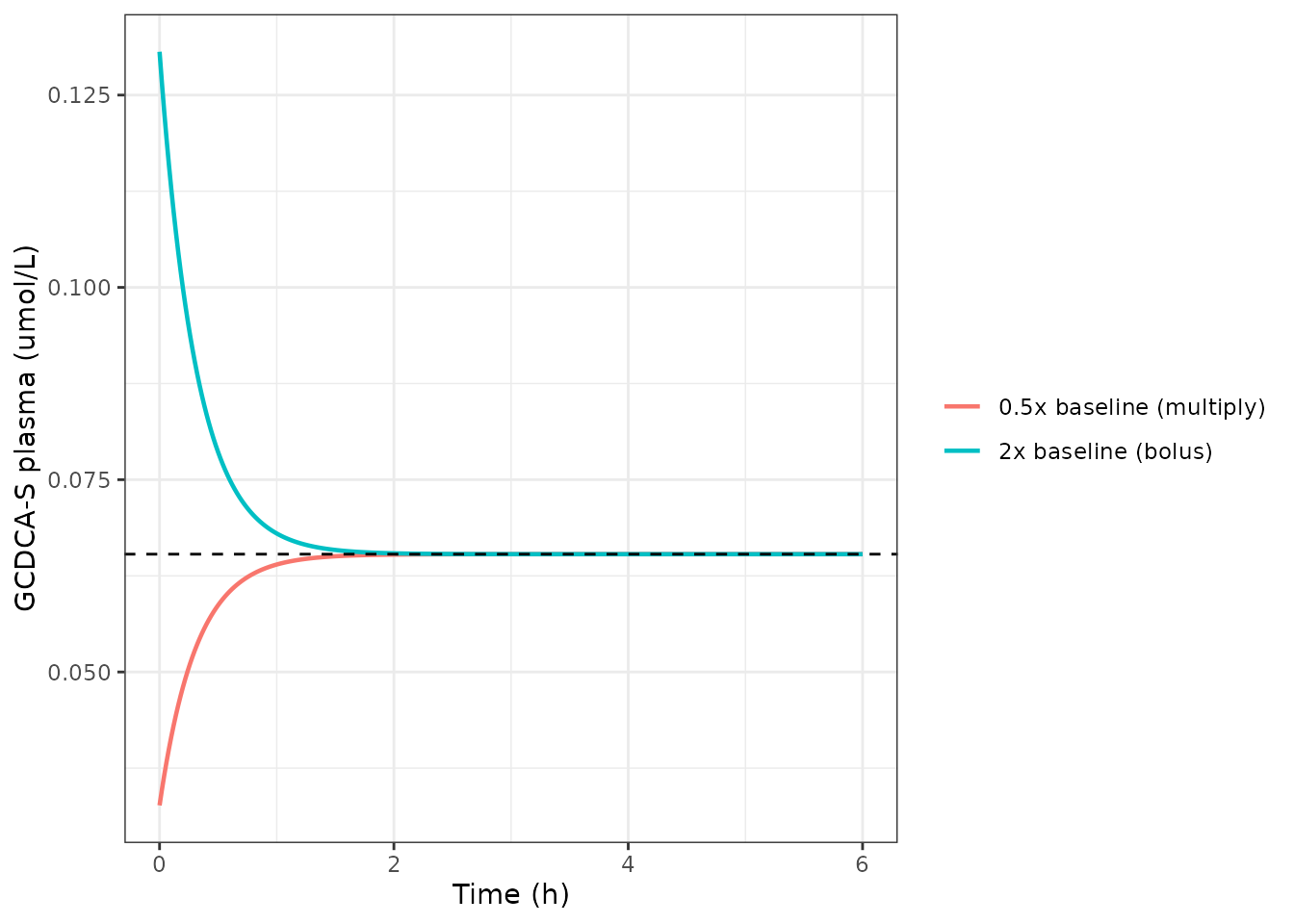
Perturbation-recovery: displacing GCDCA-S to twice and half its baseline returns it to the same steady state.
Recovery is fast because the uninhibited system’s relaxation
half-life is ln(2) * Vc / (CLh + CLR) = 0.217 h. This is a
load-bearing property of the model: under strong OATP1B3 inhibition
CLh collapses, the effective half-life lengthens by more
than an order of magnitude, and the biomarker therefore accumulates
slowly rather than jumping to a new quasi-steady state.
Mass-balance / flux check
At the baseline, production must exactly balance elimination, and the
renal fraction of the total flux is the fraction excreted in urine,
fe.
flux_in    <- ksyn
flux_hep   <- clh * css_analytic
flux_renal <- clr * css_analytic
fe         <- clr / (clh + clr)

c(production = flux_in,
  hepatobiliary = flux_hep,
  renal = flux_renal,
  net = flux_in - flux_hep - flux_renal,
  fe_percent = 100 * fe,
  biliary_percent = 100 * (1 - fe))
#>      production   hepatobiliary           renal             net      fe_percent
#>    1.000000e+00    9.797518e-01    2.024820e-02   -5.898060e-17    2.024820e+00
#> biliary_percent
#>    9.797518e+01

stopifnot(abs(flux_in - flux_hep - flux_renal) < 1e-12)
fe = 2.02% reproduces the paper’s central mechanistic
finding: biliary excretion is the primary route of elimination for
GCDCA-S (reported as ~95%, with fe < 5%; Results and
Discussion, and Table S6 which infers fe < 3.1-6.9% from
four independent clinical DDI studies).
A second, sharper identity: with no inhibitor present, the
operational renal clearance Ae(0-24) / AUC(0-24) must
recover the CLR parameter exactly.
ev_24 <- rxode2::et(seq(0, 24, by = 0.02), cmt = "Cc") |> as.data.frame()
ev_24$CONMED_PROBENECID <- 0
s24 <- rxode2::rxSolve(mod0, ev_24, returnType = "data.frame")
#> ℹ omega/sigma items treated as zero: 'etalksyn', 'etalcl_renal', 'etaltlag_rif', 'etald1_rif', 'etalcl_rif', 'etalvc_prob', 'etalcl_prob', 'etalkiu_oat3'

trapz <- function(t, y) sum(diff(t) * (head(y, -1) + tail(y, -1)) / 2)
clr_operational <- (max(s24$Ugcdcas) - min(s24$Ugcdcas)) / trapz(s24$time, s24$Cc)

c(clr_parameter = clr, clr_operational = clr_operational)
#>   clr_parameter clr_operational
#>            0.31            0.31
stopifnot(abs(clr_operational - clr) < 1e-6)
Rifampicin OATP1B3 interaction
The paper’s headline predictive check is the GCDCA-S plasma AUC ratio
(AUCR0-24h) after a single oral rifampicin dose. Reported
values: predicted AUCR of 13 at 600 mg against an
observed range of 10-16, and predicted
9.3 at 300 mg against an observed
4.3-5.9 (Results, “GCDCA-S model verification”; Table
S4 lists the 600 mg value as 13).
sim_rif <- function(mg, label) {
  ev <- if (is.na(mg)) {
    rxode2::et(seq(0, 24, by = 0.02), cmt = "Cc")
  } else {
    rxode2::et(amt = dose_umol(mg, MW_RIF), cmt = "central_rif",
               rate = -2, time = 0) |>
      rxode2::et(seq(0, 24, by = 0.02), cmt = "Cc")
  }
  ev <- as.data.frame(ev)
  ev$CONMED_PROBENECID <- 0
  out <- rxode2::rxSolve(mod0, ev, returnType = "data.frame")
  out$treatment <- label
  out$id <- 1L
  out
}

rif <- dplyr::bind_rows(
  sim_rif(NA,  "Control"),
  sim_rif(300, "RIF 300 mg"),
  sim_rif(600, "RIF 600 mg")
)
#> ℹ omega/sigma items treated as zero: 'etalksyn', 'etalcl_renal', 'etaltlag_rif', 'etald1_rif', 'etalcl_rif', 'etalvc_prob', 'etalcl_prob', 'etalkiu_oat3'
#> ℹ omega/sigma items treated as zero: 'etalksyn', 'etalcl_renal', 'etaltlag_rif', 'etald1_rif', 'etalcl_rif', 'etalvc_prob', 'etalcl_prob', 'etalkiu_oat3'
#> ℹ omega/sigma items treated as zero: 'etalksyn', 'etalcl_renal', 'etaltlag_rif', 'etald1_rif', 'etalcl_rif', 'etalvc_prob', 'etalcl_prob', 'etalkiu_oat3'
rate = -2 on the dose record is required so rxode2 uses
the modelled zero-order duration
dur(central_rif) <- d1_rif rather than treating the dose
as an instantaneous bolus.
conc_rif <- dplyr::filter(rif, !is.na(Cc))

o_conc <- PKNCA::PKNCAconc(conc_rif, Cc ~ time | id / treatment)
intervals <- data.frame(start = 0, end = 24,
                        auclast = TRUE, cmax = TRUE, tmax = TRUE)
nca_rif <- PKNCA::pk.nca(PKNCA::PKNCAdata(o_conc, intervals = intervals))
#> No dose information provided, calculations requiring dose will return NA.

nca_tab <- as.data.frame(nca_rif) |>
  dplyr::select(treatment, PPTESTCD, PPORRES) |>
  tidyr::pivot_wider(names_from = PPTESTCD, values_from = PPORRES)

auc_ctl <- nca_tab$auclast[nca_tab$treatment == "Control"]

# Published reference values joined BY KEY, never by row position, so a change
# in PKNCA's output ordering cannot silently transpose them.
published <- data.frame(
  treatment      = c("RIF 300 mg", "RIF 600 mg"),
  published_AUCR = c(9.3, 13),
  observed_AUCR  = c("4.3-5.9", "10-16")
)

aucr <- nca_tab |>
  dplyr::filter(treatment != "Control") |>
  dplyr::mutate(AUCR = auclast / auc_ctl) |>
  dplyr::inner_join(published, by = "treatment") |>
  dplyr::select(
    "Treatment"          = treatment,
    "AUC0-24h (uM*h)"    = auclast,
    "Cmax (uM)"          = cmax,
    "Simulated AUCR"     = AUCR,
    "Published AUCR"     = published_AUCR,
    "Observed AUCR"      = observed_AUCR
  )

knitr::kable(aucr, digits = 2,
caption = "GCDCA-S plasma AUC ratio after single-dose rifampicin, simulated vs. Ujihira 2025.")| Treatment | AUC0-24h (uM*h) | Cmax (uM) | Simulated AUCR | Published AUCR | Observed AUCR |
|---|---|---|---|---|---|
| RIF 300 mg | 15.52 | 1.07 | 9.9 | 9.3 | 4.3-5.9 |
| RIF 600 mg | 20.54 | 1.30 | 13.1 | 13.0 | 10-16 |
PKNCA reports “No dose information provided” because
GCDCA-S is endogenous and has no dose record; only the interval-based
auclast / cmax / tmax are
requested, none of which need a dose.
aucr_600 <- aucr[["Simulated AUCR"]][aucr$Treatment == "RIF 600 mg"]
aucr_300 <- aucr[["Simulated AUCR"]][aucr$Treatment == "RIF 300 mg"]

# 600 mg: must land inside the paper's observed range of 10-16 and within 15%
# of the paper's own predicted 13.
stopifnot(aucr_600 > 10, aucr_600 < 16, abs(aucr_600 / 13 - 1) < 0.15)
# 300 mg: must reproduce the paper's PREDICTED 9.3 within 15%. The paper is
# explicit that its own prediction overestimates the observed 4.3-5.9 here, so
# the target is the prediction, not the observation.
stopifnot(abs(aucr_300 / 9.3 - 1) < 0.15)
This is the strongest available end-to-end check on the extraction:
the AUCR is a product of the mg-to-umol conversion, the rifampicin PK
parameters, the unbound fraction fu_rif, the inhibition
constant Ki,u,OATP1B3, and the GCDCA-S clearance split. An
error in any one of them would move it.
ggplot2::ggplot(rif, ggplot2::aes(time, Cc, colour = treatment)) +
  ggplot2::geom_line(linewidth = 0.8) +
  ggplot2::labs(x = "Time (h)", y = "GCDCA-S plasma (umol/L)", colour = NULL) +
  ggplot2::theme_bw()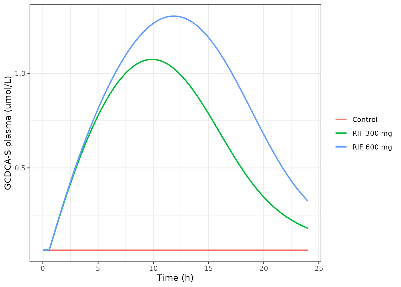
GCDCA-S plasma response to single-dose rifampicin (replicates the pattern of Ujihira 2025 Figure 3a and Figure 4b).
ggplot2::ggplot(dplyr::filter(rif, treatment != "Control"),
                ggplot2::aes(time, Cc_rif, colour = treatment)) +
  ggplot2::geom_line(linewidth = 0.8) +
  ggplot2::labs(x = "Time (h)", y = "Rifampicin plasma (umol/L)", colour = NULL) +
  ggplot2::theme_bw()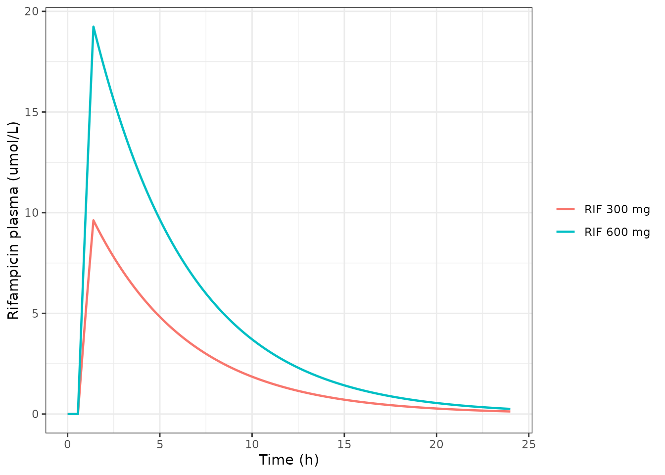
Rifampicin perpetrator PK driving the interaction (replicates Ujihira 2025 Figure 4c).
Probenecid OAT3 interaction
For OAT3 the paper’s metric is renal clearance, not plasma AUC: Table
S4 reports a CLR ratio
(CLR,+inhibitor / CLR,control) of 0.1 at
steady state under the probenecid regimen. The regimen is 500 mg at 6 pm
and 11 pm on day 0, then 500 mg at 7 am, 1 pm, 6 pm and 11 pm on days
1-7 (Table 1).
# t = 0 is the day-0 6 pm dose; the day-1 onward pattern repeats every 24 h.
dose_times <- c(0, 5, as.vector(outer(c(13, 19, 24, 29), 24 * (0:6), "+")))
dose_times <- sort(dose_times[dose_times <= 24 * 7.5])
grid <- seq(0, 24 * 7.5, by = 0.05)

sim_prob <- function(on) {
  ev <- if (on) {
    rxode2::et(amt = dose_umol(500, MW_PROB), cmt = "depot_prob",
               time = dose_times) |>
      rxode2::et(grid, cmt = "Cc")
  } else {
    rxode2::et(grid, cmt = "Cc")
  }
  ev <- as.data.frame(ev)
  ev$CONMED_PROBENECID <- as.integer(on)
  rxode2::rxSolve(mod0, ev, returnType = "data.frame")
}

prob_ctl <- sim_prob(FALSE)
#> ℹ omega/sigma items treated as zero: 'etalksyn', 'etalcl_renal', 'etaltlag_rif', 'etald1_rif', 'etalcl_rif', 'etalvc_prob', 'etalcl_prob', 'etalkiu_oat3'
prob_on  <- sim_prob(TRUE)
#> ℹ omega/sigma items treated as zero: 'etalksyn', 'etalcl_renal', 'etaltlag_rif', 'etald1_rif', 'etalcl_rif', 'etalvc_prob', 'etalcl_prob', 'etalkiu_oat3'

# Steady-state 24 h window (day 6 -> day 7).
window_metrics <- function(s) {
  k <- s$time >= 144 & s$time <= 168
  auc <- trapz(s$time[k], s$Cc[k])
  ae  <- max(s$Ugcdcas[k]) - min(s$Ugcdcas[k])
  c(AUC = auc, Ae = ae, CLR = ae / auc)
}

w_ctl <- window_metrics(prob_ctl)
w_on  <- window_metrics(prob_on)

prob_tab <- data.frame(
  Metric = c("AUC0-24h (uM*h)", "Ae0-24h (umol)", "CLR (L/h)"),
  Control = as.numeric(w_ctl),
  Probenecid = as.numeric(w_on),
  Ratio = as.numeric(w_on) / as.numeric(w_ctl)
)
knitr::kable(prob_tab, digits = 4,
caption = "GCDCA-S at steady state under the Willemin probenecid regimen.")| Metric | Control | Probenecid | Ratio |
|---|---|---|---|
| AUC0-24h (uM*h) | 1.5676 | 2.7081 | 1.7276 |
| Ae0-24h (umol) | 0.4860 | 0.1046 | 0.2153 |
| CLR (L/h) | 0.3100 | 0.0386 | 0.1246 |
clr_ratio <- unname(w_on["CLR"] / w_ctl["CLR"])
auc_ratio <- unname(w_on["AUC"] / w_ctl["AUC"])

c(clr_ratio = clr_ratio, published_clr_ratio = 0.1,
  auc_ratio = auc_ratio, X = 1.7)
#>           clr_ratio published_clr_ratio           auc_ratio                   X
#>           0.1246237           0.1000000           1.7275692           1.7000000

# Table S4 reports the CLR ratio to one significant figure as 0.1; require the
# simulated ratio to be consistent with that rounding (stated as an explicit
# interval rather than round(), which is rounding-mode dependent at 0.125).
stopifnot(clr_ratio > 0.05, clr_ratio < 0.15)
# The plasma AUC ratio must recover X = 1.7 to within 5%: CLh dominates total
# clearance, so reducing it 1.7-fold raises plasma exposure 1.7-fold, while the
# OAT3 inhibition of the small renal arm contributes almost nothing to AUC.
stopifnot(abs(auc_ratio / 1.7 - 1) < 0.05)
The two ratios separate the two mechanisms exactly as the paper
describes them (Figure S3): OAT3 inhibition is read out almost entirely
in CLR (ratio 0.125), while the plasma AUC moves only by
the concentration-independent X factor (1.73 against
X = 1.7). This is why the paper recommends CLR
rather than plasma AUC as the GCDCA-S metric for OAT3-mediated DDI.
prob_plot <- dplyr::bind_rows(
  dplyr::mutate(prob_ctl, arm = "Control"),
  dplyr::mutate(prob_on,  arm = "Probenecid 500 mg QID")
)
ggplot2::ggplot(prob_plot, ggplot2::aes(time / 24, Cc, colour = arm)) +
  ggplot2::geom_line(linewidth = 0.7) +
  ggplot2::labs(x = "Time (days)", y = "GCDCA-S plasma (umol/L)", colour = NULL) +
  ggplot2::theme_bw() +
  ggplot2::theme(legend.position = "bottom")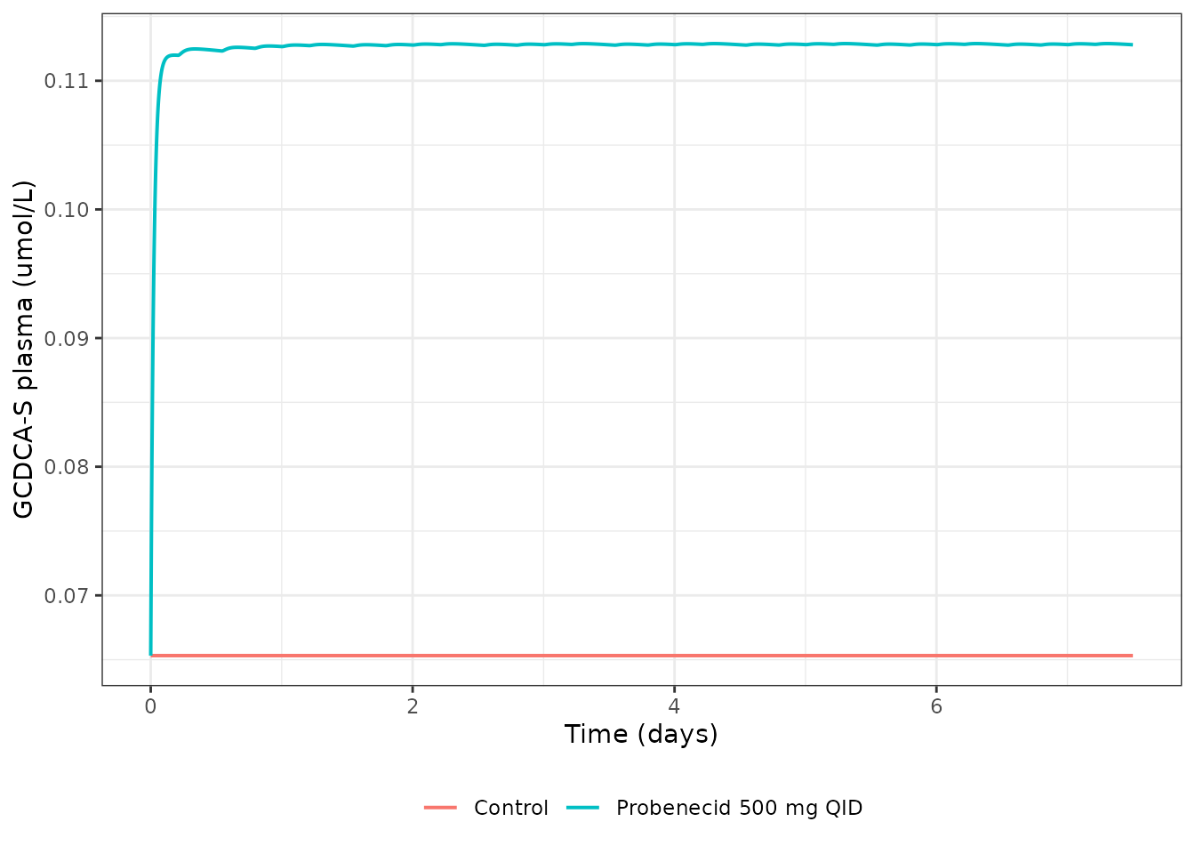
GCDCA-S plasma and renal clearance under multiple-dose probenecid (replicates the pattern of Ujihira 2025 Figure 3a-b).
Between-subject variability and the observed baseline
The paper reports an observed GCDCA-S plasma baseline of
approximately 80 nmol/L (Results) and 85 nmol/L in Table S5. The typical
value implied by the parameters is lower, at 65.32 nmol/L, because
ksyn carries 61% log-normal IIV and the reported baselines
are arithmetic means, not medians.
set.seed(20250101)
ev_cohort <- rxode2::et(seq(0, 24, by = 1), cmt = "Cc") |> as.data.frame()
ev_cohort$CONMED_PROBENECID <- 0

cohort <- rxode2::rxSolve(mod, ev_cohort, nSub = 200, returnType = "data.frame")

baseline_by_subject <- cohort |>
  dplyr::filter(time == 0) |>
  dplyr::summarise(
    median_nM = median(Cc) * 1000,
    mean_nM   = mean(Cc) * 1000,
    cv_pct    = 100 * sd(Cc) / mean(Cc)
  )
baseline_by_subject
#>   median_nM  mean_nM cv_pct
#> 1  69.49396 77.68741 57.494

# Analytic log-normal mean of the baseline: median * exp(omega^2 / 2).
c(analytic_mean_nM = css_analytic * 1000 * exp(0.3163576 / 2),
  reported_mean_nM = 80)
#> analytic_mean_nM reported_mean_nM
#>         76.51049         80.00000
The simulated cohort mean baseline lands close to the reported ~80 nmol/L, and the simulated baseline CV is consistent with the observed 34-69% range across the three development studies.
ggplot2::ggplot(dplyr::filter(cohort, time == 0),
                ggplot2::aes(Cc * 1000)) +
  ggplot2::geom_histogram(bins = 30, fill = "grey70", colour = "white") +
  ggplot2::geom_vline(xintercept = 80, linetype = "dashed") +
  ggplot2::labs(x = "Baseline GCDCA-S plasma (nmol/L)", y = "Subjects",
                caption = "Dashed line: reported observed baseline of ~80 nmol/L.") +
  ggplot2::theme_bw()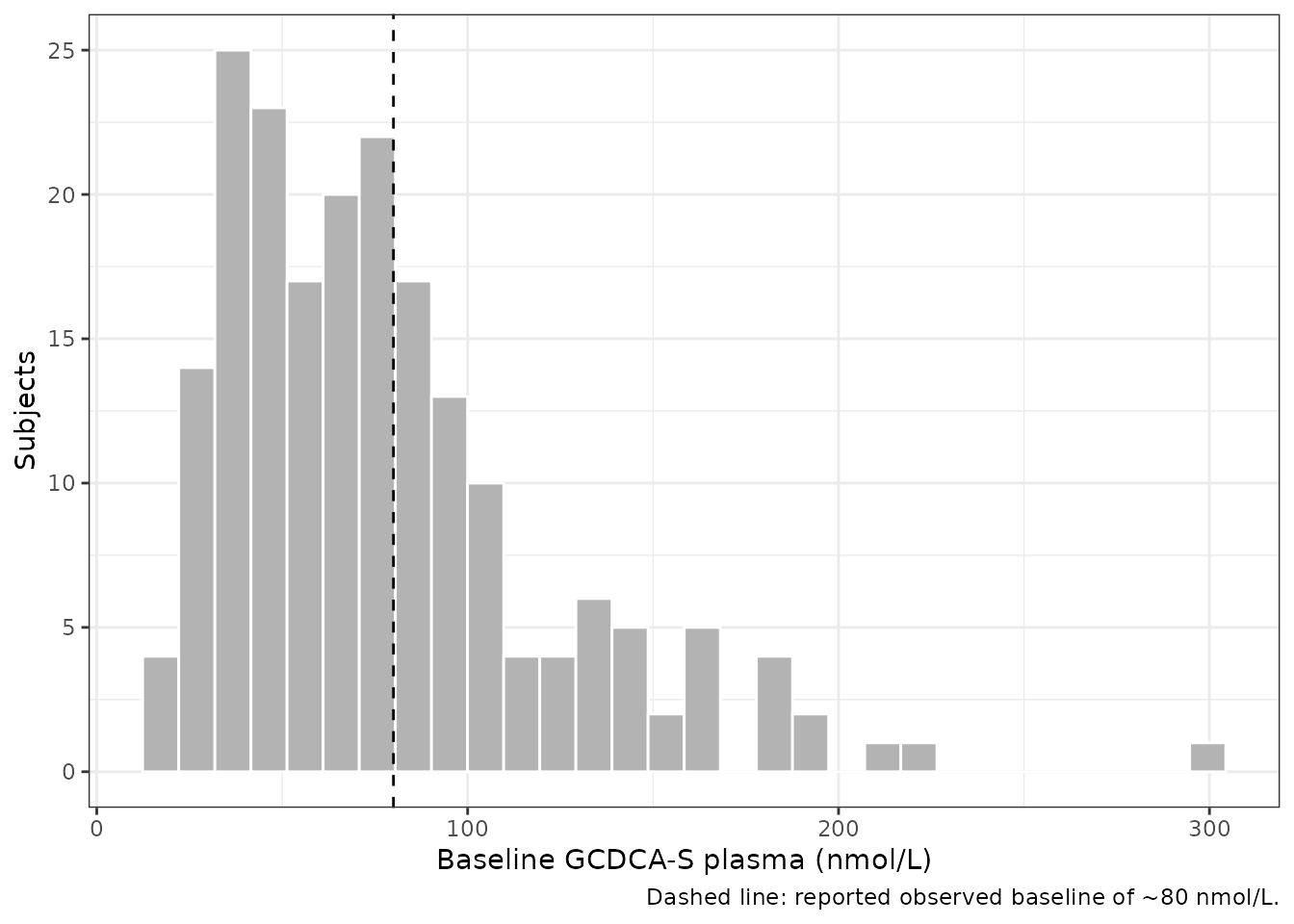
Simulated baseline GCDCA-S distribution in 200 virtual subjects, no inhibitor.
Assumptions and deviations
Unbound fractions are not reported by Ujihira 2025.
The model’s inhibition terms are driven by unbound perpetrator
concentrations (Cu,RIF, Cu,PROB), and both
inhibition constants in Table 2 are unbound constants, but neither the
main text nor Supplementary Material S1 ever states the fu
used to convert the modelled total plasma concentrations to
unbound. Both values come from the upstream models the paper explicitly
adopts, and neither is verifiable from the Ujihira 2025 sources alone.
They are therefore pinned against two published answer keys instead:
-
Rifampicin
fu= 0.11. Carried by the sibling nlmixr2lib extractionsBarnett_2018_coproporphyrin_IandBarnett_2018_rosuvastatin, whose source-trace comments record Barnett 2018 Table 1 footnote c convertingKi,total= 1.15 uM toKi,unbound= 0.13 uM and 2.23 uM to 0.25 uM atfu= 0.11. Ujihira 2025 Table S7 independently lists that same Barnett study atKi,u= 0.13 uM, so the two agree. -
Probenecid
fu= 0.062. Attributed to Ahmad 2021, the source of this model’s probenecid structure (Methods, “Structural models”). Ahmad 2021 is not among this extraction’s source files, so the attribution itself could not be checked.
The two interaction checks above are what actually pin these values, and both are published answer keys:
-
fu_rifis pinned by the rifampicin AUCR check, which reproduces Table S4’s predictedAUCR0-24hof 13 at 600 mg. That number is a product of the mg-to-umol conversion, the rifampicin PK,fu_rif,Ki,u,OATP1B3, and the GCDCA-S clearance split; a materially differentfumoves it. -
fu_probis pinned by the probenecid check, which reproduces Table S4’s steady-stateCLRratio of 0.1. Recovering 0.1 requires1 + Cu,PROB/Ki,u,OAT3of about 10. The total average steady-state concentration under 500 mg QID is1752 umol / (0.95 L/h * 6 h)= 307 uM, sofu= 0.062 givesCu= 19 uM and a ratio of 0.12 – consistent with 0.1 at one significant figure, whereasfu= 1 gives 0.009 andfu= 0.03 gives 0.23. Both alternatives are excluded.
IIV scale. Table 2’s “IIV” column is a percentage
whose scale (CV% versus the Monolix omega on the log scale)
is not stated. It is read here as CV% and converted with
omega^2 = log(1 + CV^2), matching the convention used
throughout nlmixr2lib and by the sibling
Barnett_2018_coproporphyrin_I model. The reported RSEs
support an SD-scale rather than a variance-scale reading: the
best-determined term, ksyn IIV at 61% with RSE 15%, matches
the 1/sqrt(2N) = 14.4% expected for an SD estimate at N =
24, not the sqrt(2/N) = 28.9% expected for a variance. The
residual CV%-versus-omega ambiguity changes
omega by at most about 10% relative at the largest IIV and
less elsewhere.
Molecular weights are not in the paper. Doses in the source studies are in mg while the model runs in umol, so rifampicin 822.94 g/mol and probenecid 285.34 g/mol are used for the conversion; both are already carried by the nlmixr2lib registers and agree with PubChem to four significant figures.
CL RIF units. Table 2 prints the
rifampicin clearance row as CL RIF (L). It must be L/h for
Eq. 1 to balance dimensionally, and 6.7 L/h is consistent with the 6.35
L/h of the upstream Takita 2022 rifampicin model, so the printed unit is
treated as a typographical omission of the time term.
Not implemented, because the paper excluded them from the
final model: the six diurnal-fluctuation functions applied to
ksyn (Table S2; none improved the fit, p > 0.9) and the
sex effect on ksyn (Table S3; COVSEX = 0.065
with RSE 404%, dOFV = 3). The sex covariate is recorded in the model
file’s covariatesDataExcluded metadata so the screen is
preserved without creating an unused-covariate warning.
Not implemented, because the paper did not have the
data: any effect of rifampicin or probenecid on GCDCA-S
synthesis. The paper is explicit that rifampicin may both
inhibit CYP7A1/CYP8B1 and induce SULT2A1, that this could confound the
Ki,u,OATP1B3 estimate, and that its own hypothetical
simulations (Supplementary Eqs 7-10, Figure S5) show plasma AUC is
highly sensitive to ksyn. Those hypothetical variants are
sensitivity analyses, not the fitted model, and are not extracted.
Enterohepatic recirculation is likewise excluded, consistent with the
paper’s rationale that bile-acid sulfates undergo limited intestinal
reabsorption.
Perpetrator co-administration. Rifampicin and probenecid were never given together in the source studies. The model supports both legs simultaneously, but that combination is an extrapolation beyond the fitted data.
Doses are in umol, not mg. Because the whole system
is parameterised in umol and uM, dose records for
central_rif and depot_prob must be supplied in
umol. Rifampicin doses additionally require rate = -2 so
that the modelled zero-order absorption duration is applied.