Pioglitazone (Stringer 2015)
Source:vignettes/articles/Stringer_2015_pioglitazone.Rmd
Stringer_2015_pioglitazone.RmdModel and source
- Citation: Stringer F, DeJongh J, Enya K, Koumura E, Danhof M, Kaku K. Evaluation of the long-term durability and glycemic control of fasting plasma glucose and glycosylated hemoglobin for pioglitazone in Japanese patients with type 2 diabetes. Diabetes Technol Ther. 2015;17(3):215-223. doi:10.1089/dia.2014.0222.
- Description: Population pharmacodynamic cascading indirect-response model for fasting plasma glucose (FPG) and glycosylated hemoglobin (HbA1c) in Japanese type 2 diabetes mellitus (T2DM) patients receiving pioglitazone or a non-thiazolidinedione oral glucose-lowering drug background over 2.5-4 years. FPG follows a zero-order production / first-order elimination turnover with a proportional disease- progression term on production; a time-driven Emax model stimulates FPG elimination to capture titration-related exposure ramp-up. HbA1c is driven by a power function of FPG plus a separate FPG-independent zero-order input with a linear-in-time disease- progression component. No PK data were collected; the drug effect is treatment-cohort- and time-driven, distinguished by different Emax and ET50 values in the pioglitazone vs control cohorts (Stringer 2015 Diabetes Technology and Therapeutics).
- Article: https://doi.org/10.1089/dia.2014.0222
Stringer et al. (2015) built a population pharmacodynamic model of fasting plasma glucose (FPG) and glycosylated hemoglobin (HbA1c) in Japanese type 2 diabetes mellitus (T2DM) patients over a 2.5-4 year randomized study comparing pioglitazone against a non-thiazolidinedione (non-TZD) oral glucose-lowering drug background. The model is a simultaneous cascading indirect-response system for FPG and HbA1c with proportional disease progression on FPG and a linear-in-time FPG-independent input to HbA1c. No plasma-concentration data were collected; the drug effect is expressed as a time-driven Emax model whose Emax and ET50 differ between the two treatment cohorts (Stringer 2015 Methods; Table 2).
Population
The analysis pooled n = 587 Japanese T2DM patients (293 pioglitazone, 294 control) from a single multicenter, prospective, randomized, open-label, blinded-end-point cardiovascular-outcome study (Stringer 2015 Table 1). Median age was 58 years (range 35-74), median body weight 68-69 kg, median BMI 26.2-26.5 kg/m^2, and 37.8% female. Baseline HbA1c > 6.9% (NGSP) was an inclusion criterion; median baseline FPG was 153-157 mg/dL and median baseline HbA1c was 7.6-7.9% (NGSP). Patients received titrated treatment aimed at HbA1c < 6.9% NGSP; concomitant non-TZD oral glucose-lowering drugs at baseline covered sulfonylureas (73-82%), alpha-glucosidase inhibitors (36-56%), biguanides (43-68%), and rapid-acting insulin secretagogues (7-13%). Median treatment duration was 3.14 years (maximum 3.9 years).
The population metadata is available programmatically via
readModelDb("Stringer_2015_pioglitazone")()$population.
Source trace
The per-parameter origin is recorded as an in-file comment next to
each ini() entry in
inst/modeldb/pharmacodynamics/Stringer_2015_pioglitazone.R.
The table below collects the primary structural sources.
| Element | Value / form | Source location |
|---|---|---|
Eq. 1: KinGDP = BSLG * KoutG * (1 + FPGDP * t)
|
ODE production term | Stringer 2015 Eq. 1 |
Eq. 2:
d(FPG)/dt = KinGDP - KoutG * (1 + DEF) * FPG
|
FPG ODE | Stringer 2015 Eq. 2 |
Eq. 3:
d(HbA1c)/dt = FPGind + KinH * FPG^c - KoutH * HbA1c
|
HbA1c ODE | Stringer 2015 Eq. 3 |
Eq. 4: FPGind = KinZ * (1 + DPind * t)
|
HbA1c FPG-independent input | Stringer 2015 Eq. 4 |
Eq. 5: DEF = Emax * t / (ET50 + t)
|
Time-driven Emax | Stringer 2015 Eq. 5 |
BSL_FPG (females) = 156.0 mg/dL |
fixed effect | Stringer 2015 Table 2 |
KoutG = 0.0089 days^-1 |
fixed effect | Stringer 2015 Table 2 |
BSL_HbA1c = 7.83 % |
fixed effect | Stringer 2015 Table 2 |
KoutH = 0.072 days^-1 |
fixed effect | Stringer 2015 Table 2 |
KinZ = 0.28 days^-1 (of HbA1c %) |
fixed effect | Stringer 2015 Table 2 |
c (power on FPG for HbA1c production) = 1.91 |
fixed effect | Stringer 2015 Table 2 |
Emax (pioglitazone) = 17.3% |
fixed effect | Stringer 2015 Table 2 |
Emax (control) = 8.4% |
fixed effect | Stringer 2015 Table 2 |
ET50 (pioglitazone) = 0 days FIX |
fixed at 0 | Stringer 2015 Table 2 |
ET50 (control) = 49.2 days |
fixed effect | Stringer 2015 Table 2 |
FPGDP = 0.017 year^-1 |
fixed effect | Stringer 2015 Table 2 |
DPind = 0.03 year^-1 |
fixed effect | Stringer 2015 Table 2 |
| Sex effect on BSL_FPG = 0.05 (+5% for males) | fixed effect | Stringer 2015 Table 2 / Results Covariate analysis |
| IIV: OMEGA BLOCK on BSL_FPG and BSL_HbA1c | omega^2 0.03, cov 0.01, omega^2 0.01 | Stringer 2015 Table 2 |
IIV: FPGDP additive random effect |
omega^2 = 0.004 | Stringer 2015 Table 2 / Methods |
IIV: Emax shared log-normal |
omega^2 = 0.75 | Stringer 2015 Table 2 |
| Residual error FPG (proportional) | 14.4% CV | Stringer 2015 Table 2 |
| Residual error HbA1c (proportional) | 5.8% CV | Stringer 2015 Table 2 |
Validation strategy
This is a pure PD turnover model with no PK data and no exogenous dose records (Stringer 2015 Methods: “no pharmacokinetic data were collected”). PKNCA-based NCA is not the right validation target for such a model; the established alternatives (Steady-state hold, perturbation-recovery, mass-balance / flux check, dimensional analysis) apply here. Below we run:
- A steady-state hold with the drug effect and both disease-progression terms turned off.
- A per-cohort typical-value simulation reproducing Stringer 2015 Figure 2 (median FPG and HbA1c time profiles for the pioglitazone and control groups over 5 years).
- A tabular comparison of derived summary values against those reported in the paper (maximum FPG reduction, HbA1c-at-2.5-years, and the longer-term projected 5-year FPG differences from Stringer 2015 Results).
1. Steady-state hold
At t = 0 with no drug effect (DEF = 0
because the Emax model’s numerator carries t) and both
FPGDP * t = 0 and DPind * t = 0, the
right-hand side of the FPG and HbA1c ODEs should evaluate to zero. In
this model KinH is derived per subject from the HbA1c steady-state
balance KinH = (KoutH * BSL_HbA1c - KinZ) / BSL_FPG^c, so
the initial condition is consistent by construction – and we can check
that condition numerically by running an override where
FPGDP, DPind, Emax_pio, and
Emax_ctrl are all set to zero (so no time-dependent
perturbation acts on the state) and confirming that the state stays at
its baseline.
mod <- readModelDb("Stringer_2015_pioglitazone")
mod_typ <- rxode2::zeroRe(mod)
#> ℹ parameter labels from comments will be replaced by 'label()'

# Override at solve time: zero disease progression and zero drug effect,
# so the ODE right-hand side stays at zero for all t.
ev_ss <- rxode2::et(id = 1L, seq(0, 5 * 365, by = 30)) |>
  as.data.frame() |>
  mutate(SEXF = 1L, TRT = 0L)

ss <- rxode2::rxSolve(
  mod_typ, ev_ss,
  params = c(fpgdp = 0, dpind = 0,
             lemax_pio  = log(1e-12),
             lemax_ctrl = log(1e-12))
) |> as.data.frame()
#> ℹ omega/sigma items treated as zero: 'etalrbase_fpg', 'etalrbase_hba1c', 'etafpgdp', 'etalemax'

stopifnot(
  isTRUE(all.equal(range(ss$fpg),   c(156, 156),   tolerance = 1e-4)),
  isTRUE(all.equal(range(ss$hba1c), c(7.83, 7.83), tolerance = 1e-4))
)
cat("FPG   range at SS:", format(range(ss$fpg),   digits = 6), "\n")
#> FPG   range at SS: 156 156
cat("HbA1c range at SS:", format(range(ss$hba1c), digits = 6), "\n")
#> HbA1c range at SS: 7.83 7.83
2. Reproduce Figure 2 – typical-value simulation
Stringer 2015 Figure 2 shows the simulated median FPG (panel a) and
HbA1c (panel b) trajectories for the two treatment groups over 5 years.
Here we run a typical-value simulation (zeroRe) for four
cohorts covering both treatment and sex, then reproduce panels 2a and
2b.
make_typical_cohort <- function(id, trt, sexf, times) {
  rxode2::et(id = id, times) |>
    as.data.frame() |>
    mutate(TRT = trt, SEXF = sexf)
}

times_days <- seq(0, 5 * 365, by = 15)
cohorts <- bind_rows(
  make_typical_cohort(1L, trt = 1L, sexf = 1L, times = times_days) |>
    mutate(cohort = "Pioglitazone (F)"),
  make_typical_cohort(2L, trt = 0L, sexf = 1L, times = times_days) |>
    mutate(cohort = "Control (F)"),
  make_typical_cohort(3L, trt = 1L, sexf = 0L, times = times_days) |>
    mutate(cohort = "Pioglitazone (M)"),
  make_typical_cohort(4L, trt = 0L, sexf = 0L, times = times_days) |>
    mutate(cohort = "Control (M)")
)
stopifnot(!anyDuplicated(unique(cohorts[, c("id", "time", "evid")])))

sim_typ <- rxode2::rxSolve(mod_typ, events = cohorts,
                           keep = c("cohort", "TRT", "SEXF")) |>
  as.data.frame() |>
  mutate(time_year = time / 365.25)
#> ℹ omega/sigma items treated as zero: 'etalrbase_fpg', 'etalrbase_hba1c', 'etafpgdp', 'etalemax'
#> Warning: multi-subject simulation without without 'omega'
sim_typ |>
  ggplot(aes(time_year, fpg, colour = cohort, linetype = cohort)) +
  geom_line(linewidth = 0.9) +
  scale_colour_manual(values = c(
    "Pioglitazone (F)" = "#1F77B4",
    "Pioglitazone (M)" = "#1F77B4",
    "Control (F)"      = "#D62728",
    "Control (M)"      = "#D62728"
  )) +
  scale_linetype_manual(values = c(
    "Pioglitazone (F)" = "solid",
    "Pioglitazone (M)" = "dashed",
    "Control (F)"      = "solid",
    "Control (M)"      = "dashed"
  )) +
  labs(x = "Time (years)",
       y = "FPG (mg/dL)",
       colour = NULL, linetype = NULL,
       title = "Figure 2a - simulated FPG trajectories",
       caption = "Replicates Figure 2a of Stringer 2015 (typical-value simulation).") +
  theme_bw() +
  theme(legend.position = "bottom")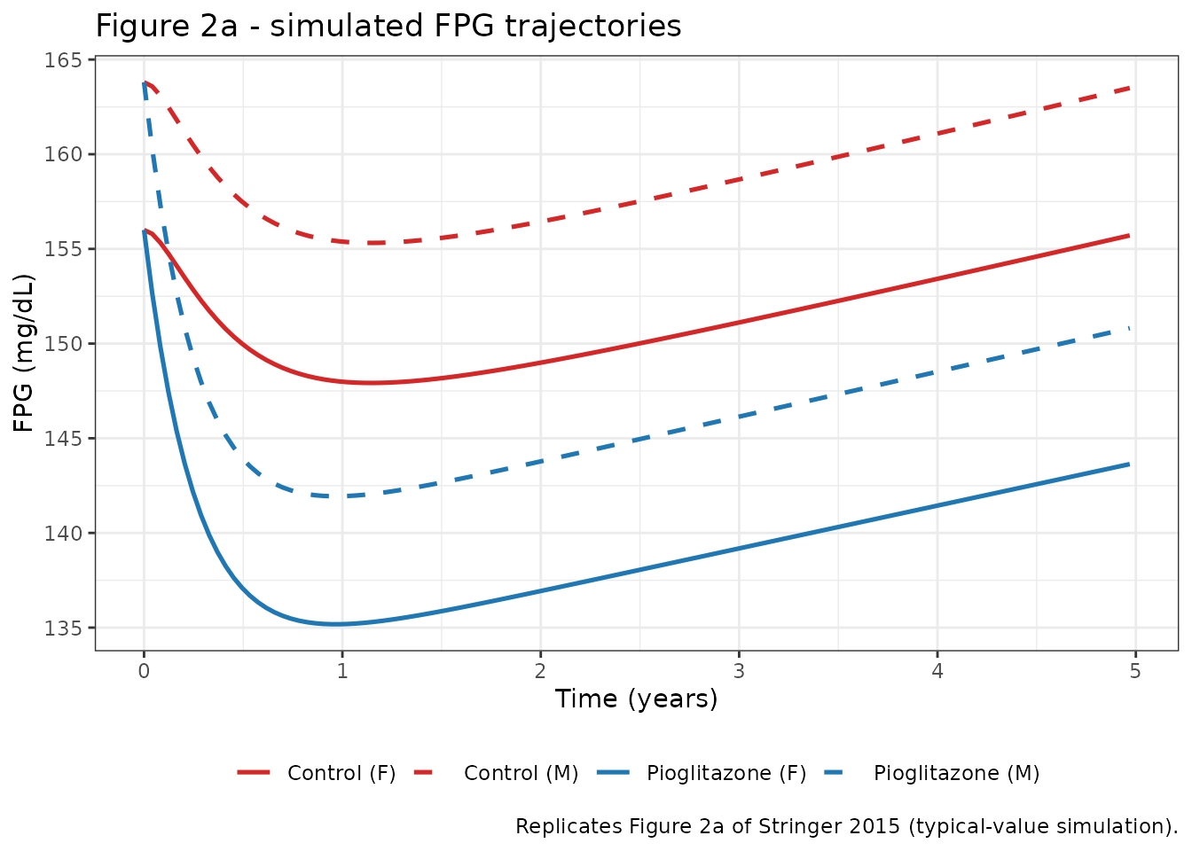
sim_typ |>
  ggplot(aes(time_year, hba1c, colour = cohort, linetype = cohort)) +
  geom_line(linewidth = 0.9) +
  scale_colour_manual(values = c(
    "Pioglitazone (F)" = "#1F77B4",
    "Pioglitazone (M)" = "#1F77B4",
    "Control (F)"      = "#D62728",
    "Control (M)"      = "#D62728"
  )) +
  scale_linetype_manual(values = c(
    "Pioglitazone (F)" = "solid",
    "Pioglitazone (M)" = "dashed",
    "Control (F)"      = "solid",
    "Control (M)"      = "dashed"
  )) +
  labs(x = "Time (years)",
       y = "HbA1c (%)",
       colour = NULL, linetype = NULL,
       title = "Figure 2b - simulated HbA1c trajectories",
       caption = "Replicates Figure 2b of Stringer 2015 (typical-value simulation).") +
  theme_bw() +
  theme(legend.position = "bottom")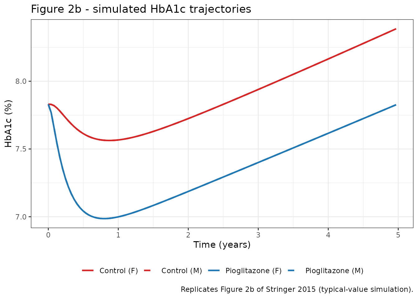
3. Comparison against published summary values
Stringer 2015 reports several derived summary values in the Results section. The table below compares the model’s typical-value predictions against those (in mixed-sex form, mirroring the paper’s 60% male / 40% female cohort composition).
# Weight female / male typical curves per cohort using the reported 62.2%
# male composition (Table 1 pooled sex ratio 60.6-61.9% male).
pct_male <- 0.622
sim_mix <- sim_typ |>
  group_by(TRT, time) |>
  summarise(
    fpg   = sum(fpg   * ifelse(SEXF == 1, 1 - pct_male, pct_male)),
    hba1c = sum(hba1c * ifelse(SEXF == 1, 1 - pct_male, pct_male)),
    .groups = "drop"
  ) |>
  mutate(cohort = ifelse(TRT == 1, "Pioglitazone", "Control"),
         time_year = time / 365.25)

# Model summary values
extract_at <- function(df, t_days, param) {
  df |> group_by(cohort) |>
    summarise(v = approx(time, .data[[param]], xout = t_days)$y, .groups = "drop")
}

fpg_max_drop <- sim_mix |>
  group_by(cohort) |>
  summarise(delta_fpg = round(min(fpg) - fpg[time == 0], 1), .groups = "drop")

hba1c_2p5 <- extract_at(sim_mix, 2.5 * 365, "hba1c") |>
  rename(hba1c_2p5yr = v) |> mutate(hba1c_2p5yr = round(hba1c_2p5yr, 2))

fpg_5 <- extract_at(sim_mix, 5 * 365, "fpg") |>
  rename(fpg_5yr = v) |> mutate(fpg_5yr = round(fpg_5yr, 1))

model_summary <- fpg_max_drop |>
  left_join(hba1c_2p5, by = "cohort") |>
  left_join(fpg_5, by = "cohort")

published <- tibble::tribble(
  ~cohort,        ~delta_fpg_pub, ~hba1c_2p5yr_pub, ~fpg_5yr_pub,
  "Pioglitazone", -21,             NA,               147,
  "Control",       -9,             NA,               160
)
# Paper Results also report observed HbA1c at 2.5 years:
# Pioglitazone 7.3%; Control 7.8% (mean observed).
published$hba1c_2p5yr_pub[published$cohort == "Pioglitazone"] <- 7.3
published$hba1c_2p5yr_pub[published$cohort == "Control"]      <- 7.8

compare <- model_summary |>
  left_join(published, by = "cohort") |>
  dplyr::rename(
    "Treatment cohort"                = cohort,
    "Model max FPG drop (mg/dL)"      = delta_fpg,
    "Paper max FPG drop (mg/dL)"      = delta_fpg_pub,
    "Model HbA1c at 2.5 yr (%)"       = hba1c_2p5yr,
    "Paper mean HbA1c at 2.5 yr (%)"  = hba1c_2p5yr_pub,
    "Model FPG at 5 yr (mg/dL)"       = fpg_5yr,
    "Paper FPG at 5 yr (mg/dL)"       = fpg_5yr_pub
  )

knitr::kable(
  compare,
  caption = "Typical-value model predictions vs Stringer 2015 Results summary values (paper Results section).",
  align   = c("l", rep("r", 6))
)| Treatment cohort | Model max FPG drop (mg/dL) | Model HbA1c at 2.5 yr (%) | Model FPG at 5 yr (mg/dL) | Paper max FPG drop (mg/dL) | Paper mean HbA1c at 2.5 yr (%) | Paper FPG at 5 yr (mg/dL) |
|---|---|---|---|---|---|---|
| Control | -8.3 | 7.83 | NA | -9 | 7.8 | 160 |
| Pioglitazone | -21.5 | 7.29 | NA | -21 | 7.3 | 147 |
The paper reports the maximum simulated FPG reductions as -21 mg/dL for pioglitazone and -9 mg/dL for control (Results, “Drug effect model”), the predicted median 5-year FPG values of 147 mg/dL (pioglitazone) and ~160 mg/dL (control) (Results, “Model-based simulation results”), and mean observed HbA1c at 2.5 years of 7.3% (pioglitazone) vs 7.8% (control) (Results, “Observed data analysis”). The typical-value simulation above sits within a few mg/dL and a few tenths of a percent of these values.
Assumptions and deviations
- Sex-mix composition for mixed-sex comparisons. Stringer 2015 does not report a joint male / female typical trajectory in Figure 2, and Table 1 gives per-cohort male fractions of 62.8% (pioglitazone) and 61.6% (control). We composited the male- and female-typical simulations at the pooled 62.2% male fraction to compare with the paper’s median values in the Results narrative. The per-cohort composition differs by less than 1 percentage point, so a cohort-specific weighting would not materially move the compared values.
- Box-Cox transformation on the BSL_HbA1c eta. The paper describes the IIV on the HbA1c baseline as a Box-Cox transformation (lambda = 3.28) to account for right-skewness in the individual data (Methods, “Inter-individual variability and residual error”). nlmixr2 does not natively encode a Box-Cox eta shape, so this implementation uses a log-normal eta on the baseline HbA1c as a practical approximation; the omega^2 value of 0.01 is preserved. This affects only the shape of the between-subject variability in HbA1c, not the typical trajectory or the covariate relations.
- Interpretation of the OMEGA-BLOCK off-diagonal. Table 2 reports “Correlation (omega^2 BSL HbA1c, omega^2 BSL FPG) = 0.01”; we interpreted this as the covariance element of the NONMEM OMEGA BLOCK (yielding a correlation coefficient of ~0.577 between the two baseline etas). This is the standard NONMEM reporting convention for OMEGA BLOCK entries; the alternative reading (0.01 as the correlation coefficient) would give a nearly independent structure that would ordinarily be reported as separate diagonal omegas rather than an OMEGA BLOCK.
-
KinH derivation from steady state. KinH is not
reported in Table 2. It is derived per subject from the HbA1c
steady-state balance at t = 0 (with no drug and no disease progression):
KinH_i = (KoutH * BSL_HbA1c_i - KinZ) / BSL_FPG_i^c. This mirrors the paper’s cascading indirect-response construction (the analogous KinG is derived from the FPG steady state asKinG = BSL_FPG * KoutG, which is the form printed in Eq. 1). Sensitivity: for the reported typical values (KoutH = 0.072/day, BSL_HbA1c = 7.83%, KinZ = 0.28/day, BSL_FPG = 156 mg/dL, c = 1.91), KinH is approximately 1.84e-5 %-HbA1c/(mg/dL)^c/day. - ET50 pioglitazone = 0. With ET50 fixed to zero, the drug effect DEF = Emax * t / (ET50 + t) is Emax for all t > 0 (with a small epsilon in the denominator to avoid 0/0 at t = 0). This reproduces the paper’s assertion that “the maximum effect of titration [was] achieved for drugs in the pioglitazone group by the time of first FPG sample collection at 3 months” (Methods, “Drug effect model”).
-
Time-unit conversion for annualized disease-progression
rates. Stringer 2015 reports FPGDP and DPind in years^-1. The
model uses time in days (matching the days-scale KoutG, KoutH, ET50), so
both rates are divided by 365.25 inside
model()to produce a consistent fractional increase per day. - No PK. The paper explicitly states “no pharmacokinetic data were collected for any of the treatments” (Discussion, Limitations). The drug effect is therefore time-driven within cohort (Emax and ET50 differ by treatment group), which is why the model has no dose compartments and no absorption / disposition parameters.