Minimal continuous-time Markov PD models (Schindler 2017)
Source:vignettes/articles/Schindler_2017_mCTMM.Rmd
Schindler_2017_mCTMM.RmdOverview
Schindler and Karlsson (2017) propose the minimal continuous-time Markov model (mCTMM) as a parsimonious reformulation of the standard CTMM for ordered-categorical PD endpoints. The key assumption is that the transition rate between any two consecutive states is independent of the state and is governed by a single mean equilibration time (MET). Under that assumption, the steady-state score probabilities follow a proportional-odds (PO) model driven by an arbitrary linear predictor (drug exposure, biomarker, time, covariates), and the CTMM transfer rate constants are given by
(paper Eqs. 8-9). The probability mass in each score state evolves via the CTMM ODEs (Eq. 6):
with boundary states carrying only one neighbour. This vignette exercises the three worked mCTMM examples from Schindler 2017:
-
Fatigue in sunitinib-treated GIST patients (four
states 0 / 1 / 2 / 3+; Table II) –
modellib("Schindler_2017_sunitinib_fatigue"). -
Hand-foot syndrome (HFS) in sunitinib-treated GIST
patients (four states 0-3; Table II) –
modellib("Schindler_2017_sunitinib_hfs"). -
Likert pain in placebo-arm diabetic-neuropathy
patients (eleven states 0-10; Table III) –
modellib("Schindler_2017_likert_pain").
For fatigue and HFS the drug-effect driver is the model-predicted
relative change from baseline in soluble vascular endothelial growth
factor receptor 3 (sVEGFR-3), which is inlined as a one-compartment
indirect-response turnover (the same simple-Imax form used in the
companion Hansson_2013a_sunitinib biomarker model). The
Likert-pain model has no drug exposure – placebo time-course and
rescue-acetaminophen use enter the cumulative-logit predictor
directly.
- Citation: Schindler E, Karlsson MO. A Minimal Continuous-Time Markov Pharmacometric Model. AAPS J. 2017;19(5):1424-1435. doi:10.1208/s12248-017-0109-1 (open access).
- Companion Schindler-lab / Karlsson-lab papers reproduced here:
- Hansson EK et al. (2013) CPT PSP 2:e85 (fatigue / HFS DTMM comparators).
- Plan EL et al. (2012) CPT 91(5):820-828 (Likert pain count-model comparator; DDMODEL00000194).
Model file structure
Each of the three model files follows the same skeleton:
- Baseline sVEGFR-3 dynamics (fatigue / HFS only) – a one-compartment
indirect-response ODE with simple-Imax inhibition of
kin3and turnover ratekout3 = 1 / MRT_SVEGFR3. Driven by the per-cycle drug-exposure summaryauc = DOSE / CLI. - Steady-state cumulative logits Pss(Y >= k) = expit(alpha_k +
linpred), where alpha_k = alpha_1 + b_2 + … + b_k (paper Eq. 11) and
linpredis the exposure driver (theta_sVEGFR3 * sVEGFR3relfor fatigue and HFS;theta_time * t_weeks + theta_ace * CONMED_PARAfor Likert; paper Eqs. 12-13). - Steady-state score probabilities Pss,k via Eq. 11.
- Transfer rate constants lambda_{k,k+1} and lambda_{k+1,k} via Eqs. 8-9.
- Probability-compartment ODEs (Eq. 6) with initial conditions set to Pss at t = 0.
- Derived expected-grade / expected-score output for typical-value visualisation.
Source trace
| Item | Value / equation | Paper location |
|---|---|---|
| PO logit | logit(P(Y >= k)) = alpha_k + f(theta, x) | Eq. 1 |
| Expit inverse | P(Y >= k) = 1 / (1 + exp(-(alpha_k + f(theta, x)))) | Eq. 2 |
| Score probability | P(Y = k) = P(Y >= k) - P(Y >= k+1) | Eq. 3 |
| CTMM ODE for P(Y = k) | dP/dt = -sum(lambda_out) * P + sum(lambda_in) * P_neighbour | Eq. 6 |
| Constant MET | MET = 1 / (lambda_{k,k+1} + lambda_{k+1,k}) | Eq. 7 |
| lambda_{k-1,k} | Pss_k / (MET * (Pss_{k-1} + Pss_k)) | Eq. 8 (rearranged) |
| lambda_{k,k-1} | Pss_{k-1} / (MET * (Pss_{k-1} + Pss_k)) | Eq. 9 |
| Pss cumulative | Pss(Y >= k) = expit(alpha_k + f(theta, x)) | Eq. 10 |
| Pss discrete | Pss_k = Pss(Y>=k) - Pss(Y>=k+1) | Eq. 11 |
| Fatigue / HFS predictor | theta_sVEGFR3 * sVEGFR3rel(t) | Eq. 12 |
| Likert predictor | theta_time * t (weeks) + theta_ace * CONMED_PARA | Eq. 13 |
| Fatigue estimates | alpha_1 -1.85; b_2 -1.08; b_3 -1.92; MET 909 h; theta_sVEGFR3 -1.87 | Table II Fatigue |
| HFS estimates | alpha_1 -17.5; b_2 -1.99; b_3 -2.66; MET 399 h; theta_sVEGFR3 -20.5 | Table II HFS |
| Likert estimates | alpha_1 9.56; b_2..b_10; MET_0 10.8 h; SlopeMET 0.740/wk; theta_time -0.141/wk; theta_ace 1.84 | Table III |
Verification: steady-state hold at baseline
At time = 0 with no drug exposure
(DOSE = 0) and no rescue-acetaminophen
(CONMED_PARA = 0), the marginal probability of each score
should equal the paper’s steady-state Pss,k computed at
linpred = 0. This is a sanity check that the compartment
initial conditions match the algebraic Pss.
mod_fatigue <- readModelDb("Schindler_2017_sunitinib_fatigue")

# Placebo cohort: DOSE = 0, so sVEGFR-3 remains at baseline and sVEGFR3rel = 0.
# Only need one long observation window to confirm the marginal probabilities
# stay locked at Pss for all t.
ev_placebo <- data.frame(
  ID          = 1L,
  TIME        = c(0, 24 * seq(0, 200, by = 20)),
  EVID        = 0L,
  AMT         = 0,
  DOSE        = 0,
  CLI         = 32.819,
  BAS_SVEGFR3 = 63900,
  MRT_SVEGFR3 = 401,
  EC50_SVEGFR3 = 1.0
)

sim_placebo <- rxode2::rxSolve(
  rxode2::zeroRe(mod_fatigue),
  events = ev_placebo,
  addDosing = FALSE
)
#> ℹ parameter labels from comments will be replaced by 'label()'
#> ℹ omega/sigma items treated as zero: 'etaalpha1', 'etatheta_svegfr3'

# Compare compartment sums (should equal 1) and marginal probabilities
sim_placebo |>
  dplyr::mutate(
    total = pscore0 + pscore1 + pscore2 + pscore3
  ) |>
  dplyr::select(time, pscore0, pscore1, pscore2, pscore3, total) |>
  head(4) |>
knitr::kable(digits = 4, caption = "Fatigue: marginal probabilities remain at Pss under placebo.")| time | pscore0 | pscore1 | pscore2 | pscore3 | total |
|---|---|---|---|---|---|
| 0 | 0.8641 | 0.0852 | 0.0429 | 0.0078 | 1 |
| 0 | 0.8641 | 0.0852 | 0.0429 | 0.0078 | 1 |
| 480 | 0.8641 | 0.0852 | 0.0429 | 0.0078 | 1 |
| 960 | 0.8641 | 0.0852 | 0.0429 | 0.0078 | 1 |
Under no exposure the ODE is at its fixed point and the four marginal
probabilities equal the paper’s Pss_k computed from alpha_k
alone. total should be identically 1 at every time point
(mass conservation).
mod_hfs <- readModelDb("Schindler_2017_sunitinib_hfs")

sim_hfs_placebo <- rxode2::rxSolve(
  rxode2::zeroRe(mod_hfs),
  events = ev_placebo,
  addDosing = FALSE
)
#> ℹ parameter labels from comments will be replaced by 'label()'
#> ℹ omega/sigma items treated as zero: 'etaalpha1', 'etatheta_svegfr3'

sim_hfs_placebo |>
  dplyr::mutate(total = pscore0 + pscore1 + pscore2 + pscore3) |>
  dplyr::select(time, pscore0, pscore1, pscore2, pscore3, total) |>
  head(4) |>
knitr::kable(digits = 6, caption = "HFS: placebo marginal probabilities.")| time | pscore0 | pscore1 | pscore2 | pscore3 | total |
|---|---|---|---|---|---|
| 0 | 1 | 0 | 0 | 0 | 1 |
| 0 | 1 | 0 | 0 | 0 | 1 |
| 480 | 1 | 0 | 0 | 0 | 1 |
| 960 | 1 | 0 | 0 | 0 | 1 |
For HFS the paper reports that ~74% of patients had grade 0 for the
entire study. Under placebo (sVEGFR3rel = 0) the alpha_1 =
-17.5 estimate gives
Pss(Y >= 1) = expit(-17.5) ~ 2.5e-8, i.e., essentially
all mass in grade 0. That matches the biological interpretation that HFS
does not occur in the absence of drug.
mod_likert <- readModelDb("Schindler_2017_likert_pain")

ev_likert_placebo <- data.frame(
  ID          = 1L,
  TIME        = 24 * seq(0, 100, by = 5),
  EVID        = 0L,
  AMT         = 0,
  CONMED_PARA = 0L
)

sim_likert_placebo <- rxode2::rxSolve(
  rxode2::zeroRe(mod_likert),
  events = ev_likert_placebo,
  addDosing = FALSE
)
#> ℹ parameter labels from comments will be replaced by 'label()'
#> ℹ omega/sigma items treated as zero: 'etaalpha1', 'etalmet0', 'etatheta_time', 'etaslopemet'

sim_likert_placebo |>
  dplyr::select(time, dplyr::starts_with("pscore"), expected_score) |>
  dplyr::mutate(total = pscore0 + pscore1 + pscore2 + pscore3 + pscore4 +
                        pscore5 + pscore6 + pscore7 + pscore8 + pscore9 + pscore10) |>
  head(3) |>
knitr::kable(digits = 4, caption = "Likert: initial marginal probabilities (t=0, no acetaminophen).")| time | pscore0 | pscore1 | pscore2 | pscore3 | pscore4 | pscore5 | pscore6 | pscore7 | pscore8 | pscore9 | pscore10 | expected_score | total |
|---|---|---|---|---|---|---|---|---|---|---|---|---|---|
| 0 | 1e-04 | 4e-04 | 0.0051 | 0.0307 | 0.1317 | 0.3470 | 0.3305 | 0.1240 | 0.0271 | 0.0029 | 4e-04 | 5.4633 | 1 |
| 120 | 1e-04 | 4e-04 | 0.0054 | 0.0324 | 0.1391 | 0.3550 | 0.3215 | 0.1173 | 0.0257 | 0.0028 | 4e-04 | 5.4241 | 1 |
| 240 | 1e-04 | 4e-04 | 0.0058 | 0.0352 | 0.1491 | 0.3638 | 0.3099 | 0.1091 | 0.0237 | 0.0026 | 4e-04 | 5.3722 | 1 |
The Likert initial-condition mass sits mainly around scores 5-6 (mid-range pain), consistent with the diabetic-neuropathy inclusion criterion of moderate-to-severe baseline pain reported by Plan 2012.
Drug-effect scenario: fatigue and HFS under 50 mg sunitinib
For the two sunitinib endpoints we simulate a stylised 50 mg/day
continuous dosing schedule (drug on from t = 0), so
sVEGFR3rel(t) drops from 0 toward its drug-driven
steady-state suppression, and the mCTMM state probabilities shift toward
higher grades.
ev_drug <- data.frame(
  ID          = 1L,
  TIME        = 24 * seq(0, 200, by = 5),
  EVID        = 0L,
  AMT         = 0,
  DOSE        = 50,
  CLI         = 32.819,
  BAS_SVEGFR3 = 63900,
  MRT_SVEGFR3 = 401,
  EC50_SVEGFR3 = 1.0
)

sim_fat_drug <- rxode2::rxSolve(rxode2::zeroRe(mod_fatigue), events = ev_drug, addDosing = FALSE)
#> ℹ parameter labels from comments will be replaced by 'label()'
#> ℹ omega/sigma items treated as zero: 'etaalpha1', 'etatheta_svegfr3'
sim_hfs_drug <- rxode2::rxSolve(rxode2::zeroRe(mod_hfs),    events = ev_drug, addDosing = FALSE)
#> ℹ parameter labels from comments will be replaced by 'label()'
#> ℹ omega/sigma items treated as zero: 'etaalpha1', 'etatheta_svegfr3'

marginals_fat <- sim_fat_drug |>
  dplyr::select(time, pscore0, pscore1, pscore2, pscore3) |>
  tidyr::pivot_longer(-time, names_to = "score", values_to = "prob") |>
  dplyr::mutate(
    endpoint = "Fatigue",
    score = factor(gsub("pscore", "grade ", score), levels = paste0("grade ", 0:3))
  )
marginals_hfs <- sim_hfs_drug |>
  dplyr::select(time, pscore0, pscore1, pscore2, pscore3) |>
  tidyr::pivot_longer(-time, names_to = "score", values_to = "prob") |>
  dplyr::mutate(
    endpoint = "HFS",
    score = factor(gsub("pscore", "grade ", score), levels = paste0("grade ", 0:3))
  )

ggplot(dplyr::bind_rows(marginals_fat, marginals_hfs),
       aes(x = time / 24, y = prob, colour = score)) +
  geom_line(size = 0.9) +
  facet_wrap(~endpoint) +
  labs(x = "Time (days)", y = "Marginal probability",
       title = "Marginal state probabilities under 50 mg/day sunitinib",
       colour = "Score") +
  scale_y_continuous(limits = c(0, 1))
#> Warning: Using `size` aesthetic for lines was deprecated in ggplot2 3.4.0.
#> ℹ Please use `linewidth` instead.
#> This warning is displayed once per session.
#> Call `lifecycle::last_lifecycle_warnings()` to see where this warning was
#> generated.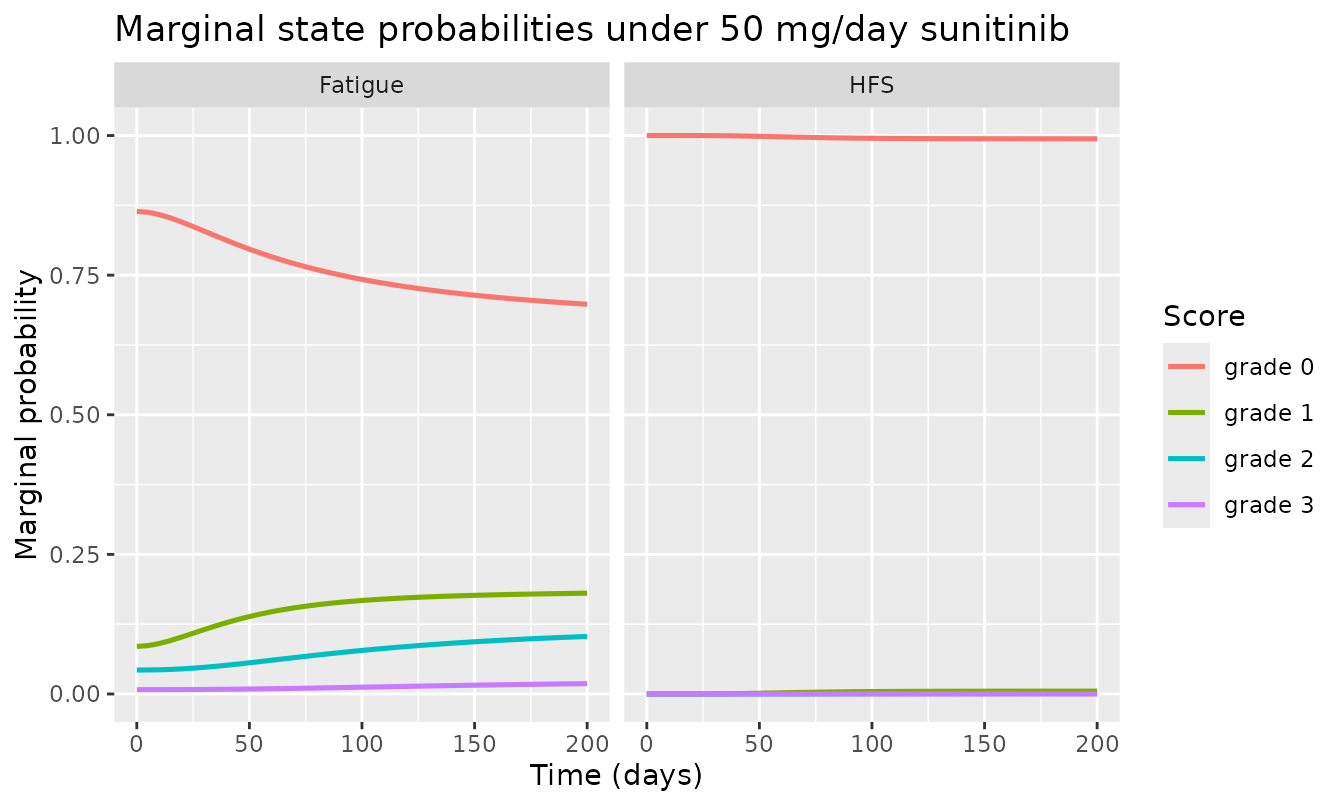
Consistent with the paper’s narrative and the DTMM sibling model
(Hansson_2013_sunitinib_hfs), the marginal probability of
grades > 0 rises over the first few weeks of sunitinib dosing as
sVEGFR-3 is depleted, then plateaus at the mCTMM-implied steady state.
Fatigue has a much shorter MET (909 h vs 399 h for HFS actually – see
the paper: MET for HFS is smaller than for fatigue, meaning HFS
transitions more quickly; note however that alpha_1 for HFS is deeply
negative so the steady-state probability shifts massively only under
strong sVEGFR-3 suppression).
Likert scenario: placebo time-course and acetaminophen effect
For Likert we compare two placebo scenarios: no rescue medication
(CONMED_PARA = 0) and continuous acetaminophen use
(CONMED_PARA = 1).
ev_likert_noace <- data.frame(
  ID = 1L, TIME = 24 * seq(0, 84, by = 3), EVID = 0L, AMT = 0, CONMED_PARA = 0L
)
ev_likert_ace <- ev_likert_noace |> dplyr::mutate(CONMED_PARA = 1L)

sim_likert_noace <- rxode2::rxSolve(rxode2::zeroRe(mod_likert), events = ev_likert_noace, addDosing = FALSE)
#> ℹ parameter labels from comments will be replaced by 'label()'
#> ℹ omega/sigma items treated as zero: 'etaalpha1', 'etalmet0', 'etatheta_time', 'etaslopemet'
sim_likert_ace   <- rxode2::rxSolve(rxode2::zeroRe(mod_likert), events = ev_likert_ace,   addDosing = FALSE)
#> ℹ parameter labels from comments will be replaced by 'label()'
#> ℹ omega/sigma items treated as zero: 'etaalpha1', 'etalmet0', 'etatheta_time', 'etaslopemet'

expected_score_df <- dplyr::bind_rows(
  sim_likert_noace |> dplyr::select(time, expected_score) |>
    dplyr::mutate(scenario = "Placebo (no rescue)"),
  sim_likert_ace   |> dplyr::select(time, expected_score) |>
    dplyr::mutate(scenario = "Placebo + acetaminophen daily")
)

ggplot(expected_score_df, aes(x = time / 24, y = expected_score, colour = scenario)) +
  geom_line(size = 0.9) +
  labs(x = "Time (days)", y = "Expected Likert score (0-10)",
       title = "Likert-pain typical trajectory under placebo",
       colour = NULL) +
  scale_y_continuous(limits = c(0, 10))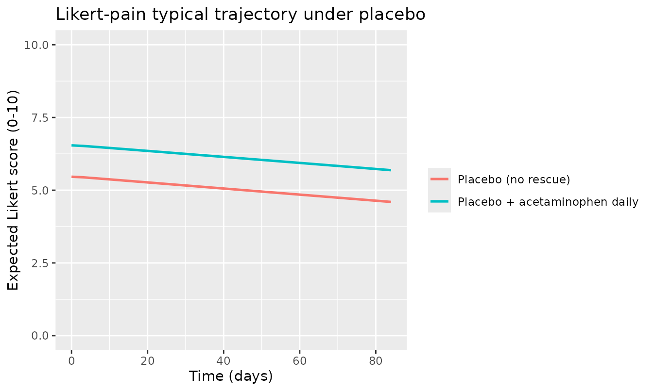
The placebo arm shows the paper’s expected mild time-related pain
reduction (negative theta_time = -0.141/week).
Acetaminophen use shifts the expected score upward – as the paper’s
Discussion notes, acetaminophen is a rescue medication taken because of
pain, so the positive theta_ace = 1.84 coefficient reflects
reverse causality, not a pro-nociceptive drug effect. The
MET(t) = MET_0 * (1 + SlopeMET * t_weeks) schedule
increases score stability progressively over the 84-day follow-up.
Assumptions and deviations
-
Simulation semantics – marginal-probability ODE, not Markov
chain sampling. The mCTMM as fitted by NONMEM under
$ESTIMATION LAPLACE LIKEis a Markov chain where the state at each observation resets the compartment amounts (observed score to 1, all others to 0). Between observations the ODEs evolve the probability of each possible next score. The rxode2 models in this vignette simulate only the marginal-probability trajectory (no observation-time state reset), which faithfully reproduces the population- averaged proportion in each state over time but does not capture the within-subject serial correlation (the point of the Markov model). Users who need proper within-subject Markov-chain trajectories can wrap the ODE simulation in an outer sampling loop: sample the observed score at each observation time from the compartment amounts, then reset the compartments before continuing. -
Between-subject variability (BSV) – declared but the parser
rejects chained cumulative-logit expressions. The Schindler
2017 fit reports additive BSV on
alpha_1for all three models plus exponential BSV ontheta_sVEGFR3(fatigue / HFS) or onMET_0,theta_time, andSlopeMET(Likert). The paper’s omega values (as standard deviations, per the Table II and Table III footnote text) are:- Fatigue: omega(alpha_1) = 0.770 (RSE 19%); omega(theta_sVEGFR3) = 1.07 (RSE 7.7%).
- HFS: omega(alpha_1) = 11.2 (RSE 90%; note the paper’s explicit discussion of the alpha_1 identifiability challenge because HFS grades > 0 are essentially absent without drug); omega(theta_sVEGFR3) = 0.475 (RSE 28%).
- Likert: omega(alpha_1) = 3.19 (RSE 4.6%); omega(MET_0) = 0.881 (RSE
6.8%); omega(theta_time) = 0.241 (RSE 4.9%); omega(SlopeMET) = 2.15 (RSE
7.7%). These are declared as etas (
etaalpha1 ~ variance, …) in each model file and the individual parameters are constructed via mu-referenced variables (alpha1_ind,theta_sv,met0_ind,slopemet_ind). To satisfy rxode2 5.1.3’s mu-reference syntax parser – which rejects barealpha_1 + b_2combinations – the subsequent cumulative-logit b_k terms are wrapped in parentheses (alpha1_ind + (b2) + (b3) + ...). This is a purely cosmetic AST transformation and does not affect the numerical semantics.
-
Pss_kguardeps = 1e-12. The transfer-rate expressions (Eqs. 8-9) divide byMET * (Pss_k + Pss_{k+1}). At extreme covariate values (very large positive or very large negativelinpred), a Pss pair could collapse to zero and trigger a divide-by-zero. A tinyepsfloor is added in the denominator to keep the ODE solver stable; the effect is negligible when the Pss values are non-degenerate. -
Placeholder additive residual error on the expected-grade /
expected- score output. The Schindler 2017 fit uses NONMEM’s
LIKElikelihood option and has no observation-error model. To let nlmixr2 build these model files at all, a placeholderadd(0.5)residual is attached to the continuousexpected_grade/expected_scoreoutput. This does NOT affect the marginal-probability trajectory itself and can be ignored during simulation-only use. Users fitting these models to data should replace the placeholder with a proper categorical likelihood (see the source paper’s Supplementary NONMEM code for the LIKE-based form). -
Time-varying MET functional form (Likert). The
paper reports “a linear increase in MET with a typical slope (SlopeMET)
estimated to be 0.740 week^-1”; Eq. 13 gives Pss but does not print
MET(t) explicitly. This vignette and the model file encode the
linear-fractional form
MET(t) = MET_0 * (1 + SlopeMET * t_weeks)(dimensionally consistent with SlopeMET’s1/weekunit). An alternative additive formMET(t) = MET_0 + SlopeMET_h_per_week * t_weekswas considered but discarded because the paper’s SlopeMET unit is1/week(dimensionless slope), noth/week. -
Upstream sVEGFR-3 turnover parameters (fatigue and
HFS). The
sVEGFR3rel(t)driver is generated inline from a one-compartment indirect-response turnover with simple-Imax inhibition ofkin3, parameterised byBAS_SVEGFR3,MRT_SVEGFR3, andEC50_SVEGFR3(per-subject posthoc inputs from the upstream Hansson 2013a fit; DDMODEL00000197). Schindler 2017 cites this upstream biomarker model (their reference 17) but does not report its parameters. The vignette virtual cohort uses the Hansson 2013a typical values (63,900 pg/mL, 401 h, 1.0 mg*h/L) as documented inmodellib("Hansson_2013a_sunitinib"). -
Compare-against-published values. The paper reports
Table I “average number of transitions per individual” as a
discriminative summary between mCTMM, PO, and DTMM / count fits.
Reproducing this metric requires a proper within-subject Markov-chain
simulation (score sampling + state reset at each observation) rather
than the marginal-probability ODE shown here. Users who need this metric
can layer that sampling loop on top of
rxSolve()output; the required compartment amounts are already exposed aspscore0 ... pscore10.