Anti-HBV siRNA HBsAg turnover MBMA in mice (Sandra 2024) • nlmixr2lib

Model and source

Citation: Sandra L, T’jollyn H, Vermeulen A, Ackaert O, Perez-Ruixo JJ. Model-based meta-analysis to quantify the effects of short interfering RNA therapeutics on hepatitis B surface antigen turnover in hepatitis B-infected mice. CPT Pharmacometrics Syst Pharmacol. 2024;13(5):729-742. doi:10.1002/psp4.13129
Description: MBMA. Preclinical (mouse). Kinetic-pharmacodynamic (K-PD) model coupled to an inhibitory indirect response model (IRM) for the baseline- and placebo-corrected serum hepatitis B surface antigen (HBsAg) time course after a single dose of an anti-HBV short interfering RNA (siRNA) in HBV-infected mice. Fitted by model-based meta-analysis to 237 study-arm-mean HBsAg observations digitised from 25 active treatment arms in 9 placebo- or vehicle-controlled non-clinical studies, covering 13 siRNAs in 3 delivery classes: N-acetylgalactosamine-conjugated (GalNAc), lipid-nanoparticle formulated (LNP), and cholesterol-conjugated (chol, all co-administered with a GalNAc-conjugated melittin-like endolytic peptide). The dose enters a virtual biophase compartment depot_kpd as an absolute amount in ng and decays at the first-order rate kel; the amount in depot_kpd inhibits synthesis of the response through a sigmoid Imax term with drug-specific id50 and hill. kel is siRNA-CLASS specific (GalNAc 0.03291, LNP 0.1368, chol 0.2403 /day, i.e. biophase half-lives of 21.06, 5.07 and 2.89 days); id50 is siRNA-SPECIFIC and spans 41.46 ng (chol NAG-MLP chol-siHBV-74+77) to 7451 ng (GalNAc VIR-2218); hill was estimated for the 3 siRNAs with more than one dose level and FIXED to 1 for the other 10. The single system parameter kdeg (0.7196 /day) is shared across all siRNAs and carries the only random effect, a BETWEEN-STUDY variance (CV 31.4%). The output Cc is the double-corrected HBsAg ratio: it starts at exactly 1 (ksyn = kdeg, so the response is at steady state before treatment) and falls toward 0 as the siRNA suppresses HBsAg synthesis; it is NOT a drug concentration. Suitable simulation scope is the study-arm-mean HBsAg ratio time course, NOT individual-mouse HBsAg and NOT plasma or liver siRNA pharmacokinetics – the paper notes that a K-PD biophase amount cannot be extrapolated back to plasma PK because siRNA plasma and liver kinetics are completely temporally disconnected.
Article: https://doi.org/10.1002/psp4.13129

Sandra 2024 is a model-based meta-analysis (MBMA) that pools published hepatitis B surface antigen (HBsAg) time-course data from HBV-infected mice in order to compare the potency and the duration of response of anti-HBV short interfering RNA (siRNA) therapeutics across three delivery classes. Note that the journal tags the article “Systematic Review”: it does contain a PubMed literature search and a CONSORT diagram, but it is not a model-cataloguing review. The authors digitised the primary data and fitted their own NONMEM model to it, and Table 3 of the paper reports that model’s original parameter estimates. That fitted model is what this vignette validates.

The structure is a kinetic-pharmacodynamic (K-PD) biophase compartment driving an inhibitory indirect response model (IRM). Because a K-PD model infers biophase kinetics from the pharmacodynamic data alone, there is no measured siRNA concentration anywhere in this model, and the paper is explicit that the biophase amount cannot be extrapolated back to plasma pharmacokinetics: siRNA plasma and liver kinetics are completely temporally disconnected.

Population

The analysis dataset pooled nine placebo- or vehicle-controlled non-clinical studies, contributing 237 mean HBsAg observations from 25 active treatment arms and 13 distinct siRNAs (Sandra 2024 Table 1 and Results). Four studies came from the PubMed search, three from the EASL 2022 abstract book, and two from publicly available business presentations and reports. Sandra 2024 Table 1 has ten rows but nine distinct studies, because Amy C.H. Lee 2018 (reference 40) contributed two separate experiments; summing its n study column over the ten rows gives 147 animals.

Two murine HBV models were represented. Hydrodynamic-injection (HDI) mice received 10 to 13.5 ug of the pHBV1.3 plasmid through the tail vein and were dosed 21 days post-infection; these were NOD-SCID mice, 6 to 8 weeks old, female where sex was reported. AAV-HBV mice received an AAV2/8 or AAV8 vector carrying the HBV genome at 1e11 vector genomes and were dosed 28 days post-infection; strain was C57BL/6 where reported and not available for several of the abstract and business-report sources. Published doses ranged from 0.03 to 9 mg/kg, given intravenously for the cholesterol-conjugated and lipid-nanoparticle siRNAs and subcutaneously for the GalNAc-conjugated siRNAs.

The same information is available programmatically via rxode2::rxode(readModelDb("Sandra_2024_siRNA_hbsag_mouse_mbma"))$population.

Source trace

Structural equations

The dependent variable is the baseline- and placebo-corrected mean HBsAg, which Sandra 2024 writes as d2HBsAg and builds in three steps. Each arm is first normalised to its own baseline (Eqs 2 and 3), then the treatment arm is divided by its concurrent control arm (Eq 4):

$\Delta \mathrm{HBsAg}_{T}(t) = \frac{\mathrm{HBsAg}_{T}(t)}{\mathrm{HBsAg}_{T}(0)}, \qquad \Delta \mathrm{HBsAg}_{C}(t) = \frac{\mathrm{HBsAg}_{C}(t)}{\mathrm{HBsAg}_{C}(0)}, \qquad \Delta^{2}\mathrm{HBsAg}(t) = \frac{\Delta \mathrm{HBsAg}_{T}(t)}{\Delta \mathrm{HBsAg}_{C}(t)}$

The double correction is why the model output starts at exactly 1 and is dimensionless. The paper gives three reasons for it: about half the included studies reported only relative HBsAg and so had no absolute baseline; the reported units were inconsistent across studies and the assay-dependent conversion factors were not published; and the correction isolates the drug-induced effect from the placebo effect.

The dose enters a virtual biophase compartment as a bolus and decays first order (Eq 5); the biophase amount inhibits the synthesis of the response through a sigmoid Imax term (Eqs 6 and 7):

$\frac{dK}{dt} = -\mathrm{KDE} \cdot K, \quad K(0) = \mathrm{Dose} \qquad \frac{d\,\Delta^{2}\mathrm{HBsAg}}{dt} = k_{syn}(1 - E) - k_{deg}\,\Delta^{2}\mathrm{HBsAg} \qquad E = \frac{K^{\gamma}}{\mathrm{ID}_{50}^{\gamma} + K^{\gamma}}$

Because the data are baseline- and placebo-corrected, the response is assumed to be at steady state before treatment, so ksyn / kdeg = 1 and therefore ksyn = kdeg; ksyn is not a separate estimated parameter and the initial condition of the response is exactly 1.

Between-study variability is log-normal on the study-level parameter (Eq 8), and the residual is additive on the log scale with a weight built from each arm’s observed variability and size (Eq 9):

$\theta_{i} = \theta_{pop}\,e^{\eta_{\theta,i}} \qquad \log \Delta^{2}\mathrm{HBsAg}_{i,j,t} = \log \widehat{\Delta^{2}\mathrm{HBsAg}}_{i,j,t} + \frac{\mathrm{CV\%}_{i,j,t}}{\sqrt{N_{i,j,t}-1}} \cdot \epsilon_{i,j,t}$

Parameter provenance

Every value below is also carried as an in-file comment beside its ini() entry in inst/modeldb/therapeuticArea/Sandra_2024_siRNA_hbsag_mouse_mbma.R.

Equation / parameter	Value	Source location
`d/dt(depot_kpd) = -kel * depot_kpd`, `depot_kpd(0) = Dose`	n/a	Sandra 2024 Eq 5
`d/dt(effect) = ksyn * (1 - inh) - kdeg * effect`	n/a	Sandra 2024 Eq 6
`inh = depot_kpd^hill / (id50^hill + depot_kpd^hill)`	n/a	Sandra 2024 Eq 7
`effect(0) = 1`, `ksyn = kdeg`	n/a	Sandra 2024 Structural model text below Eq 6
`lkdeg`	0.7196 /day (RSE 12.50%)	Table 3, `kdeg`
`lkel_galnac`	0.03291 /day (RSE 8.80%)	Table 3, `KDE GalNAc`
`lkel_lnp`	0.1368 /day (RSE 9.53%)	Table 3, `KDE LNP`
`lkel_chol`	0.2403 /day (RSE 4.86%)	Table 3, `KDE chol`
`lid50_olx703a`	2581 ng (RSE 37.09%)	Table 3, `ID50,GalNAc`
`lid50_ab729`	4435 ng (RSE 30.50%)	Table 3, `ID50,GalNAc`
`lid50_alg125755`	6287 ng (RSE 16.52%)	Table 3, `ID50,GalNAc`
`lid50_alg125819`	7426 ng (RSE 15.60%)	Table 3, `ID50,GalNAc`
`lid50_vir2218`	7451 ng (RSE 28.69%)	Table 3, `ID50,GalNAc`
`lid50_arb1740`	72.01 ng (RSE 41.37%)	Table 3, `ID50,LNP`
`lid50_arb1467`	124.0 ng (RSE 53.57%)	Table 3, `ID50,LNP`
`lid50_sihbv74_77`	41.46 ng (RSE 34.05%)	Table 3, `ID50,chol`
`lid50_arc520`	44.01 ng (RSE 34.59%)	Table 3, `ID50,chol`
`lid50_sihbv74`	48.97 ng (RSE 26.37%)	Table 3, `ID50,chol`
`lid50_sihbv75`	166.9 ng (RSE 37.15%)	Table 3, `ID50,chol`
`lid50_sihbv77`	274.0 ng (RSE 32.58%)	Table 3, `ID50,chol`
`lid50_sihbv76`	275.4 ng (RSE 33.97%)	Table 3, `ID50,chol`
`lhill_ab729`	2.547 (RSE 17.53%)	Table 3, `gamma`
`lhill_arb1740`	2.03 (RSE 13.50%)	Table 3, `gamma`
`lhill_sihbv77`	1.313 (RSE 10.31%)	Table 3, `gamma`
`lhill_other`	1, FIXED	Table 3 heading, `gamma (1 FIX all except)`
`eta_study_lkdeg`	CV 31.4% (RSE 30.8%), variance 0.3139^2	Table 3 `BSV kdeg`; Table 2 final row, 31.39
`expSd`	3.42% (RSE 4.68%)	Table 3, `RV`

Dimensional analysis

Sandra 2024 mixes an absolute biophase amount in ng with a dimensionless response ratio, so the two ODE lines carry different units and it is worth writing them out.

Term	Units	Check
`depot_kpd`	ng	biophase amount, dosed as an absolute ng amount
`kel`	1/day	class-specific
`kel * depot_kpd`	ng/day	matches `d/dt(depot_kpd)` = ng/day
`id50`	ng	same units as `depot_kpd`, so `depot_kpd/id50` is dimensionless
`hill`	dimensionless	exponent, so `(depot_kpd/id50)^hill` stays dimensionless
`inh`	dimensionless	a fraction between 0 and 1
`effect`	dimensionless	ratio of ratios (Eq 4)
`ksyn`, `kdeg`	1/day	equal to one another by the steady-state assumption
`ksyn * (1 - inh)`	1/day	matches `d/dt(effect)` = 1/day, since `effect` is dimensionless
`kdeg * effect`	1/day	matches

Because id50 and depot_kpd are both amounts in ng, a dose expressed in mg/kg must be converted with the animal’s bodyweight before it is used here. Sandra 2024 used the reported mean bodyweight where available and assumed 20 g otherwise, so a 3 mg/kg dose becomes 3 * 0.020 = 0.06 mg = 60,000 ng.

Why this vignette does not use PKNCA

The package convention is to validate with a PKNCA non-compartmental analysis. That is not applicable here. This is a K-PD model: there is no drug concentration in the model at all, and the single output is a dimensionless HBsAg ratio that starts at its maximum of 1 and falls. Cmax, Tmax, AUC and half-life of the output would not correspond to any quantity Sandra 2024 reports. The validations below follow the endogenous / mechanistic pattern instead: a steady-state hold, a parameter round-trip, closed-form identities, perturbation recovery, and reproduction of the three published simulation results.

Every simulation in this vignette is deterministic – rxode2::zeroRe() removes both the between-study random effect and the residual, matching the “deterministic simulations” the paper used for its Figures 4, 5 and 6. That means the assertions below can be exact: none of them depends on a drawn cohort, so none of them is subject to the thread-count-dependent RNG spread that makes cohort-extreme assertions unreliable in CI.

mod <- rxode2::rxode(readModelDb("Sandra_2024_siRNA_hbsag_mouse_mbma"))
#> ℹ parameter labels from comments will be replaced by 'label()'
modDet <- rxode2::zeroRe(mod)

# Sandra 2024 Tables 1 and 3: the 13 siRNAs, their delivery class, and the
# published potency and Hill exponent for each.
sirna <- tibble::tribble(
  ~drug,                        ~column,          ~class,   ~id50_paper, ~hill_paper,
  "OLX703A",                    "TRT_OLX703A",    "GalNAc",     2581,      1,
  "AB-729",                     "TRT_AB729",      "GalNAc",     4435,      2.547,
  "ALG-125755",                 "TRT_ALG125755",  "GalNAc",     6287,      1,
  "ALG-125819",                 "TRT_ALG125819",  "GalNAc",     7426,      1,
  "VIR-2218",                   "TRT_VIR2218",    "GalNAc",     7451,      1,
  "ARB-1740",                   "TRT_ARB1740",    "LNP",          72.01,   2.03,
  "ARB-1467",                   "TRT_ARB1467",    "LNP",         124.0,    1,
  "NAG-MLP chol-siHBV-74 + 77", "TRT_SIHBV74_77", "chol",         41.46,   1,
  "ARC-520",                    "TRT_ARC520",     "chol",         44.01,   1,
  "NAG-MLP chol-siHBV-74",      "TRT_SIHBV74",    "chol",         48.97,   1,
  "NAG-MLP chol-siHBV-75",      "TRT_SIHBV75",    "chol",        166.9,    1,
  "NAG-MLP chol-siHBV-77",      "TRT_SIHBV77",    "chol",        274.0,    1.313,
  "NAG-MLP chol-siHBV-76",      "TRT_SIHBV76",    "chol",        275.4,    1
)

# Sandra 2024 Table 3 and Results: class-specific KDE and the biophase
# half-lives the paper derives from them as ln(2)/KDE.
kdePaper   <- c(GalNAc = 0.03291, LNP = 0.1368, chol = 0.2403)
thalfPaper <- c(GalNAc = 21.06,   LNP = 5.07,   chol = 2.89)

trtColumns <- sirna$column

# One covariate vector selecting a single siRNA: exactly one indicator is 1.
covsFor <- function(column, columns = trtColumns) {
  out <- rep(0, length(columns))
  names(out) <- columns
  out[[column]] <- 1
  out
}

# Single-dose deterministic solve for one siRNA. `dose` is an absolute ng
# amount. as.numeric() strips any names -- rxode2::et() rejects a named amt.
solveSingle <- function(column, dose, times) {
  ev <- rxode2::et(amt = as.numeric(dose), cmt = "depot_kpd", time = 0)
  ev <- rxode2::et(ev, times)
  rxode2::rxSolve(modDet, ev, params = covsFor(column), returnType = "data.frame")
}

# Multiple-dose deterministic solve at inter-dose interval `tau`.
solveMultiple <- function(column, dose, tau, times, until = 365) {
  doseTimes <- seq(0, until, by = tau)
  doseTimes <- doseTimes[doseTimes < until]
  ev <- rxode2::et(amt = as.numeric(dose), cmt = "depot_kpd", time = doseTimes)
  ev <- rxode2::et(ev, times)
  rxode2::rxSolve(modDet, ev, params = covsFor(column), returnType = "data.frame")
}

# Area over the response curve: the paper's AOC summary metric, the integral of
# (1 - response) over the follow-up, by the trapezoidal rule.
aoc <- function(time, response) {
  sum(diff(time) * (head(1 - response, -1) + tail(1 - response, -1)) / 2)
}

Validation 1: the untreated response holds at its baseline

Because the dependent variable is baseline- and placebo-corrected, and because ksyn = kdeg was imposed rather than fitted, an untreated profile must sit at exactly 1 forever. This is the check that catches a sign error in the indirect response line, a ksyn that is not tied to kdeg, or an initial condition that was not set to 1.

ssSolve <- solveSingle("TRT_AB729", dose = 0, times = seq(0, 365, by = 1))
#> ℹ omega/sigma items treated as zero: 'eta_study_lkdeg'

stopifnot(
  # Deterministic, closed-form: no tolerance beyond floating-point noise.
  max(abs(ssSolve$Cc - 1)) < 1e-8,
  max(abs(ssSolve$effect - 1)) < 1e-8
)

c(min = min(ssSolve$Cc), max = max(ssSolve$Cc))
#> min max 
#>   1   1

Validation 2: per-siRNA parameters round-trip through the indicator wiring

The model selects one of 13 potencies and one of three elimination rates from the treatment indicators. A mis-wired indicator would silently give a neighbouring compound’s potency, so each of the 13 is solved in turn and the id50, hill and kel the model actually used are compared against the printed Table 3 values.

roundTrip <- lapply(seq_len(nrow(sirna)), function(i) {
  s <- solveSingle(sirna$column[i], dose = 1000, times = c(0, 1))
  tibble::tibble(
    drug       = sirna$drug[i],
    class      = sirna$class[i],
    id50_model = s$id50[1],
    hill_model = s$hill[1],
    kel_model  = s$kel[1]
  )
})
#> ℹ omega/sigma items treated as zero: 'eta_study_lkdeg'
#> ℹ omega/sigma items treated as zero: 'eta_study_lkdeg'
#> ℹ omega/sigma items treated as zero: 'eta_study_lkdeg'
#> ℹ omega/sigma items treated as zero: 'eta_study_lkdeg'
#> ℹ omega/sigma items treated as zero: 'eta_study_lkdeg'
#> ℹ omega/sigma items treated as zero: 'eta_study_lkdeg'
#> ℹ omega/sigma items treated as zero: 'eta_study_lkdeg'
#> ℹ omega/sigma items treated as zero: 'eta_study_lkdeg'
#> ℹ omega/sigma items treated as zero: 'eta_study_lkdeg'
#> ℹ omega/sigma items treated as zero: 'eta_study_lkdeg'
#> ℹ omega/sigma items treated as zero: 'eta_study_lkdeg'
#> ℹ omega/sigma items treated as zero: 'eta_study_lkdeg'
#> ℹ omega/sigma items treated as zero: 'eta_study_lkdeg'
roundTrip <- dplyr::bind_rows(roundTrip) |>
  dplyr::mutate(
    id50_paper = sirna$id50_paper,
    hill_paper = sirna$hill_paper,
    kel_paper  = unname(kdePaper[sirna$class])
  )

stopifnot(
  max(abs(roundTrip$id50_model - roundTrip$id50_paper)) < 1e-6,
  max(abs(roundTrip$hill_model - roundTrip$hill_paper)) < 1e-6,
  max(abs(roundTrip$kel_model  - roundTrip$kel_paper))  < 1e-9
)

roundTrip |>
  dplyr::select(
    "siRNA" = drug, "Class" = class,
    "ID50 model (ng)" = id50_model, "ID50 Table 3 (ng)" = id50_paper,
    "gamma model" = hill_model, "gamma Table 3" = hill_paper,
    "KDE model (1/day)" = kel_model
  ) |>
  knitr::kable(digits = 5)

siRNA	Class	ID50 model (ng)	ID50 Table 3 (ng)	gamma model	gamma Table 3	KDE model (1/day)
OLX703A	GalNAc	2581.00	2581.00	1.000	1.000	0.03291
AB-729	GalNAc	4435.00	4435.00	2.547	2.547	0.03291
ALG-125755	GalNAc	6287.00	6287.00	1.000	1.000	0.03291
ALG-125819	GalNAc	7426.00	7426.00	1.000	1.000	0.03291
VIR-2218	GalNAc	7451.00	7451.00	1.000	1.000	0.03291
ARB-1740	LNP	72.01	72.01	2.030	2.030	0.13680
ARB-1467	LNP	124.00	124.00	1.000	1.000	0.13680
NAG-MLP chol-siHBV-74 + 77	chol	41.46	41.46	1.000	1.000	0.24030
ARC-520	chol	44.01	44.01	1.000	1.000	0.24030
NAG-MLP chol-siHBV-74	chol	48.97	48.97	1.000	1.000	0.24030
NAG-MLP chol-siHBV-75	chol	166.90	166.90	1.000	1.000	0.24030
NAG-MLP chol-siHBV-77	chol	274.00	274.00	1.313	1.313	0.24030
NAG-MLP chol-siHBV-76	chol	275.40	275.40	1.000	1.000	0.24030

Validation 3: the effect is exactly half-maximal at the biophase ID50

Sandra 2024 Figure 4 plots the relative effect against biophase amount with a vertical line at ID50 for each class. Eq 7 makes this a closed-form identity: E = 1/2 when K = ID50, for any Hill exponent. Dosing ten times the ID50 and observing at ln(10)/KDE puts the biophase amount at exactly the ID50, so the inhibition at that moment must be 0.5 for all 13 compounds. This exercises id50, kel and hill together.

halfMax <- lapply(seq_len(nrow(sirna)), function(i) {
  kelI <- unname(kdePaper[sirna$class[i]])
  tHalfMax <- log(10) / kelI
  s <- solveSingle(sirna$column[i],
                   dose = 10 * sirna$id50_paper[i],
                   times = c(tHalfMax))
  tibble::tibble(
    drug        = sirna$drug[i],
    class       = sirna$class[i],
    biophase_ng = s$depot_kpd[1],
    id50_ng     = s$id50[1],
    inhibition  = s$inh[1]
  )
})
#> ℹ omega/sigma items treated as zero: 'eta_study_lkdeg'
#> ℹ omega/sigma items treated as zero: 'eta_study_lkdeg'
#> ℹ omega/sigma items treated as zero: 'eta_study_lkdeg'
#> ℹ omega/sigma items treated as zero: 'eta_study_lkdeg'
#> ℹ omega/sigma items treated as zero: 'eta_study_lkdeg'
#> ℹ omega/sigma items treated as zero: 'eta_study_lkdeg'
#> ℹ omega/sigma items treated as zero: 'eta_study_lkdeg'
#> ℹ omega/sigma items treated as zero: 'eta_study_lkdeg'
#> ℹ omega/sigma items treated as zero: 'eta_study_lkdeg'
#> ℹ omega/sigma items treated as zero: 'eta_study_lkdeg'
#> ℹ omega/sigma items treated as zero: 'eta_study_lkdeg'
#> ℹ omega/sigma items treated as zero: 'eta_study_lkdeg'
#> ℹ omega/sigma items treated as zero: 'eta_study_lkdeg'
halfMax <- dplyr::bind_rows(halfMax)

stopifnot(
  # Biophase amount has decayed to exactly the ID50 ...
  max(abs(halfMax$biophase_ng / halfMax$id50_ng - 1)) < 1e-4,
  # ... so the sigmoid Imax term must be exactly one half.
  # Realised 3.3e-6 and 8.4e-7 -- these bounds sit ~30x above the lsoda
  # integration error accumulated over the (up to 70 day) decay, and far
  # below any real defect: the closest neighbouring ID50 in Table 3 is 18%
  # away, so a mis-wired indicator moves these by four orders of magnitude.
  max(abs(halfMax$inhibition - 0.5)) < 1e-4
)

halfMax |>
  dplyr::select("siRNA" = drug, "Class" = class,
                "Biophase (ng)" = biophase_ng, "ID50 (ng)" = id50_ng,
                "Inhibition E" = inhibition) |>
  knitr::kable(digits = 4)

siRNA	Class	Biophase (ng)	ID50 (ng)	Inhibition E
OLX703A	GalNAc	2581.0085	2581.00	0.5
AB-729	GalNAc	4435.0053	4435.00	0.5
ALG-125755	GalNAc	6287.0207	6287.00	0.5
ALG-125819	GalNAc	7426.0244	7426.00	0.5
VIR-2218	GalNAc	7451.0245	7451.00	0.5
ARB-1740	LNP	72.0100	72.01	0.5
ARB-1467	LNP	124.0000	124.00	0.5
NAG-MLP chol-siHBV-74 + 77	chol	41.4600	41.46	0.5
ARC-520	chol	44.0100	44.01	0.5
NAG-MLP chol-siHBV-74	chol	48.9700	48.97	0.5
NAG-MLP chol-siHBV-75	chol	166.9000	166.90	0.5
NAG-MLP chol-siHBV-77	chol	274.0000	274.00	0.5
NAG-MLP chol-siHBV-76	chol	275.4001	275.40	0.5

Reproducing Figure 4, the relative effect as a function of biophase amount for one representative compound of each class:

figure4Drugs <- c("ALG-125755", "ARB-1467", "NAG-MLP chol-siHBV-74")
figure4 <- sirna |>
  dplyr::filter(drug %in% figure4Drugs) |>
  dplyr::rowwise() |>
  dplyr::reframe({
    kVals <- 10^seq(0, 6, length.out = 200)
    tibble::tibble(
      drug  = drug,
      class = class,
      id50  = id50_paper,
      K     = kVals,
      E     = kVals^hill_paper / (id50_paper^hill_paper + kVals^hill_paper)
    )
  })

ggplot(figure4, aes(x = K, y = E, colour = class)) +
  geom_line(linewidth = 0.9) +
  geom_vline(
    data = dplyr::distinct(figure4, class, id50),
    aes(xintercept = id50, colour = class), linetype = "dashed"
  ) +
  scale_x_log10() +
  labs(
    x = "Amount at biophase K (ng)",
    y = "Relative effect E",
    colour = "siRNA class"
  ) +
  theme_bw()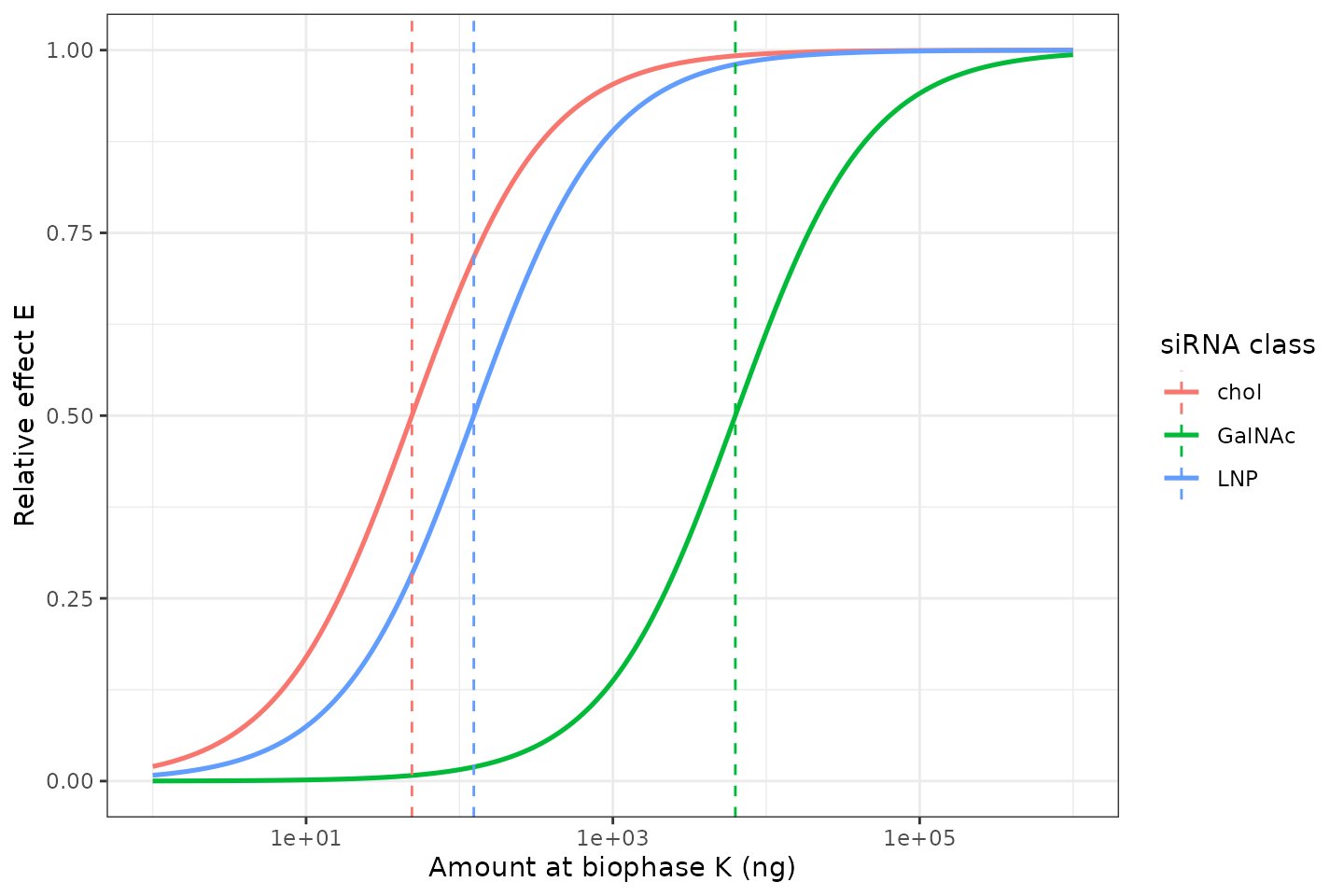

Replicates Figure 4 of Sandra 2024: relative effect E as a function of biophase amount K, stratified by siRNA class. Vertical lines mark each compound’s ID50, where E is exactly 0.5.

Validation 4: biophase half-lives reproduce the published values

Sandra 2024 Results states that the three KDE estimates correspond to biophase elimination half-lives of 21.06, 5.07 and 2.89 days for GalNAc, LNP and cholesterol siRNAs. The half-life is measured back off the simulated biophase decay rather than recomputed from the same kel the model was given, so this gate can actually go red if a class indicator selects the wrong rate.

halfLife <- lapply(c("GalNAc", "LNP", "chol"), function(cls) {
  column <- sirna$column[sirna$class == cls][1]
  s <- solveSingle(column, dose = 1e5, times = seq(0, 120, by = 0.01))
  # Time at which the simulated biophase amount first falls to half the dose.
  idx <- which(s$depot_kpd <= 0.5 * 1e5)[1]
  tibble::tibble(
    class          = cls,
    thalf_sim      = s$time[idx],
    thalf_paper    = unname(thalfPaper[cls])
  )
})
#> ℹ omega/sigma items treated as zero: 'eta_study_lkdeg'
#> ℹ omega/sigma items treated as zero: 'eta_study_lkdeg'
#> ℹ omega/sigma items treated as zero: 'eta_study_lkdeg'
halfLife <- dplyr::bind_rows(halfLife) |>
  dplyr::mutate(pct_diff = 100 * (thalf_sim - thalf_paper) / thalf_paper)

stopifnot(
  # The paper rounds to 2 decimal places, and the observation grid is 0.01 day,
  # so agreement to 0.1% is the resolution of the comparison, not a loose bound.
  # A wrong class rate would move these by a factor of 4 or more.
  max(abs(halfLife$pct_diff)) < 0.5
)

halfLife |>
  dplyr::select("Class" = class, "t1/2 simulated (day)" = thalf_sim,
                "t1/2 Sandra 2024 (day)" = thalf_paper,
                "% difference" = pct_diff) |>
  knitr::kable(digits = 3)

Class	t1/2 simulated (day)	t1/2 Sandra 2024 (day)	% difference
GalNAc	21.07	21.06	0.047
LNP	5.07	5.07	0.000
chol	2.89	2.89	0.000

The response itself turns over much faster than any of the biophase compartments: ln(2)/kdeg is 0.963 days, so HBsAg recovery is limited by how long siRNA persists in the biophase, not by HBsAg kinetics. That is the mechanistic point of the paper.

Validation 5: single-dose simulations reproduce the Figure 5 class ordering

Sandra 2024 Figure 5 simulates a single dose at 1, 10, 100 and 1000 times each compound’s ID50 with one year of follow-up, and summarises the nadir (as the maximal log drop) and the area over the curve (AOC). The Results state that GalNAc-siRNAs showed a more profound HBsAg decline than LNP- and cholesterol-siRNAs, “as demonstrated by the larger nadir and AOC across all simulated ID50-fold dose levels”.

doseFold <- c(1, 10, 100, 1000)
obsGrid <- seq(0, 365, by = 0.5)

singleDose <- lapply(seq_len(nrow(sirna)), function(i) {
  lapply(doseFold, function(fold) {
    s <- solveSingle(sirna$column[i],
                     dose = fold * sirna$id50_paper[i],
                     times = obsGrid)
    tibble::tibble(
      drug  = sirna$drug[i],
      class = sirna$class[i],
      fold  = fold,
      time  = s$time,
      Cc    = s$Cc
    )
  }) |> dplyr::bind_rows()
}) |> dplyr::bind_rows()
#> ℹ omega/sigma items treated as zero: 'eta_study_lkdeg'
#> ℹ omega/sigma items treated as zero: 'eta_study_lkdeg'
#> ℹ omega/sigma items treated as zero: 'eta_study_lkdeg'
#> ℹ omega/sigma items treated as zero: 'eta_study_lkdeg'
#> ℹ omega/sigma items treated as zero: 'eta_study_lkdeg'
#> ℹ omega/sigma items treated as zero: 'eta_study_lkdeg'
#> ℹ omega/sigma items treated as zero: 'eta_study_lkdeg'
#> ℹ omega/sigma items treated as zero: 'eta_study_lkdeg'
#> ℹ omega/sigma items treated as zero: 'eta_study_lkdeg'
#> ℹ omega/sigma items treated as zero: 'eta_study_lkdeg'
#> ℹ omega/sigma items treated as zero: 'eta_study_lkdeg'
#> ℹ omega/sigma items treated as zero: 'eta_study_lkdeg'
#> ℹ omega/sigma items treated as zero: 'eta_study_lkdeg'
#> ℹ omega/sigma items treated as zero: 'eta_study_lkdeg'
#> ℹ omega/sigma items treated as zero: 'eta_study_lkdeg'
#> ℹ omega/sigma items treated as zero: 'eta_study_lkdeg'
#> ℹ omega/sigma items treated as zero: 'eta_study_lkdeg'
#> ℹ omega/sigma items treated as zero: 'eta_study_lkdeg'
#> ℹ omega/sigma items treated as zero: 'eta_study_lkdeg'
#> ℹ omega/sigma items treated as zero: 'eta_study_lkdeg'
#> ℹ omega/sigma items treated as zero: 'eta_study_lkdeg'
#> ℹ omega/sigma items treated as zero: 'eta_study_lkdeg'
#> ℹ omega/sigma items treated as zero: 'eta_study_lkdeg'
#> ℹ omega/sigma items treated as zero: 'eta_study_lkdeg'
#> ℹ omega/sigma items treated as zero: 'eta_study_lkdeg'
#> ℹ omega/sigma items treated as zero: 'eta_study_lkdeg'
#> ℹ omega/sigma items treated as zero: 'eta_study_lkdeg'
#> ℹ omega/sigma items treated as zero: 'eta_study_lkdeg'
#> ℹ omega/sigma items treated as zero: 'eta_study_lkdeg'
#> ℹ omega/sigma items treated as zero: 'eta_study_lkdeg'
#> ℹ omega/sigma items treated as zero: 'eta_study_lkdeg'
#> ℹ omega/sigma items treated as zero: 'eta_study_lkdeg'
#> ℹ omega/sigma items treated as zero: 'eta_study_lkdeg'
#> ℹ omega/sigma items treated as zero: 'eta_study_lkdeg'
#> ℹ omega/sigma items treated as zero: 'eta_study_lkdeg'
#> ℹ omega/sigma items treated as zero: 'eta_study_lkdeg'
#> ℹ omega/sigma items treated as zero: 'eta_study_lkdeg'
#> ℹ omega/sigma items treated as zero: 'eta_study_lkdeg'
#> ℹ omega/sigma items treated as zero: 'eta_study_lkdeg'
#> ℹ omega/sigma items treated as zero: 'eta_study_lkdeg'
#> ℹ omega/sigma items treated as zero: 'eta_study_lkdeg'
#> ℹ omega/sigma items treated as zero: 'eta_study_lkdeg'
#> ℹ omega/sigma items treated as zero: 'eta_study_lkdeg'
#> ℹ omega/sigma items treated as zero: 'eta_study_lkdeg'
#> ℹ omega/sigma items treated as zero: 'eta_study_lkdeg'
#> ℹ omega/sigma items treated as zero: 'eta_study_lkdeg'
#> ℹ omega/sigma items treated as zero: 'eta_study_lkdeg'
#> ℹ omega/sigma items treated as zero: 'eta_study_lkdeg'
#> ℹ omega/sigma items treated as zero: 'eta_study_lkdeg'
#> ℹ omega/sigma items treated as zero: 'eta_study_lkdeg'
#> ℹ omega/sigma items treated as zero: 'eta_study_lkdeg'
#> ℹ omega/sigma items treated as zero: 'eta_study_lkdeg'

singleSummary <- singleDose |>
  dplyr::group_by(drug, class, fold) |>
  dplyr::summarise(
    nadir_logdrop = -log10(min(Cc)),
    aoc           = aoc(time, Cc),
    .groups = "drop"
  )

ggplot(singleDose, aes(x = time, y = Cc, group = drug, colour = class)) +
  geom_line(linewidth = 0.6) +
  facet_wrap(~ paste0(fold, "x ID50")) +
  scale_y_log10() +
  labs(
    x = "Time (day)",
    y = expression(Delta^2 * "HBsAg (fraction of baseline)"),
    colour = "siRNA class"
  ) +
  theme_bw()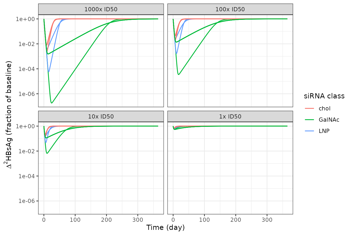

Replicates Figure 5a of Sandra 2024: deterministic single-dose simulations at 1, 10, 100 and 1000 times ID50, one curve per siRNA, coloured by class, over one year of follow-up.

Figure 5 plots one curve per compound and stratifies them by colour, so the class-level claim is a statement about the envelope of each class’s curves. Both the envelope (the class maximum) and the class median are computed below, because they do not agree and the disagreement is informative.

classOrder <- singleSummary |>
  dplyr::group_by(fold, class) |>
  dplyr::summarise(
    nadir_max    = max(nadir_logdrop),
    nadir_median = median(nadir_logdrop),
    aoc_max      = max(aoc),
    aoc_median   = median(aoc),
    .groups = "drop"
  ) |>
  tidyr::pivot_wider(
    names_from  = class,
    values_from = c(nadir_max, nadir_median, aoc_max, aoc_median)
  )

stopifnot(
  # Sandra 2024 Results, on the envelope of Figure 5: GalNAc gives the larger
  # nadir than both other classes at EVERY simulated ID50-fold dose level, and
  # the classes rank GalNAc > LNP > chol. Realised nadir maxima are
  # 0.27/0.21/0.18, 2.18/1.32/0.80, 4.46/2.77/1.67 and 6.74/4.24/2.58 at
  # 1/10/100/1000x ID50. Deterministic, so this is a property of the parameter
  # set, not of a drawn cohort.
  all(classOrder$nadir_max_GalNAc > classOrder$nadir_max_LNP),
  all(classOrder$nadir_max_LNP    > classOrder$nadir_max_chol),
  # The AOC ordering holds on BOTH the envelope and the median, at every dose.
  all(classOrder$aoc_max_GalNAc    > classOrder$aoc_max_LNP),
  all(classOrder$aoc_max_LNP       > classOrder$aoc_max_chol),
  all(classOrder$aoc_median_GalNAc > classOrder$aoc_median_LNP),
  all(classOrder$aoc_median_LNP    > classOrder$aoc_median_chol),
  # Nadir on the class median holds against chol at every dose level.
  all(classOrder$nadir_median_GalNAc > classOrder$nadir_median_chol),
  # Both metrics rise with dose (Figure 5b,c show a near-linear increase).
  all(diff(classOrder$nadir_max_GalNAc) > 0),
  all(diff(classOrder$aoc_median_GalNAc) > 0)
)

classOrder |>
  dplyr::select(
    "ID50-fold dose"    = fold,
    "Nadir max, GalNAc" = nadir_max_GalNAc,
    "Nadir max, LNP"    = nadir_max_LNP,
    "Nadir max, chol"   = nadir_max_chol,
    "AOC med, GalNAc"   = aoc_median_GalNAc,
    "AOC med, LNP"      = aoc_median_LNP,
    "AOC med, chol"     = aoc_median_chol
  ) |>
  knitr::kable(digits = 2)

ID50-fold dose	Nadir max, GalNAc	Nadir max, LNP	Nadir max, chol	AOC med, GalNAc	AOC med, LNP	AOC med, chol
1	0.26	0.21	0.18	21.05	3.77	2.88
10	2.18	1.32	0.80	72.85	17.18	9.97
100	4.46	2.77	1.67	140.20	33.69	19.19
1000	6.74	4.24	2.58	209.72	50.48	28.74

One comparison does not reproduce on the class median, and it is not gated. Taking the median nadir within each class instead of the envelope, GalNAc falls below LNP at 10x, 100x and 1000x ID50 (0.95 vs 1.05, 1.86 vs 2.17, 2.81 vs 3.32), although it stays above cholesterol everywhere. The mechanism is the Hill exponent rather than anything about delivery class: gamma was estimated for only three compounds and fixed to 1 for the other ten, and at doses above ID50 a gamma near 2 deepens the nadir far more than the biophase half-life does. The LNP class has just two members, one of which (ARB-1740, gamma = 2.03) drags its two-point median upward, whereas the GalNAc median lands on a compound with gamma fixed to 1 – its own high-gamma member, AB-729 (gamma = 2.547), produces the deepest nadir of all 13 compounds at 6.74 log at 1000x ID50 but sits above the median. The class-median nadir is therefore an artefact of which compounds happened to have multiple dose levels available for estimating gamma, not a property of the classes, and the envelope reading is the one that corresponds to Figure 5. The AOC comparison, which is driven by the biophase half-life and is the paper’s duration-of-response argument, is unaffected and holds on both summaries.

singleSummary |>
  dplyr::group_by(fold, class) |>
  dplyr::summarise(nadir_median = median(nadir_logdrop), .groups = "drop") |>
  tidyr::pivot_wider(names_from = class, values_from = nadir_median) |>
  dplyr::mutate(`GalNAc > LNP?` = ifelse(GalNAc > LNP, "yes", "NO")) |>
  dplyr::rename("ID50-fold dose" = fold) |>
  knitr::kable(digits = 3)

ID50-fold dose	GalNAc	LNP	chol	GalNAc > LNP?
1	0.265	0.191	0.180	yes
10	0.946	1.049	0.668	NO
100	1.859	2.168	1.360	NO
1000	2.810	3.316	2.100	NO

Validation 6: multiple-dose regimens reproduce the published dosing counts

This is the paper’s headline quantitative claim and the tightest gate in this vignette. Sandra 2024 selected the inter-dose interval to match each class’s biophase half-life and reports that reaching a given log drop and AOC target over one year required 126, 72 and 17 dosing occasions for cholesterol-, LNP- and GalNAc-siRNAs respectively (Results and Figure 6). Those three integers are a joint function of all three KDE estimates, so a single mis-transcribed rate breaks at least one of them.

tauModel <- log(2) / kdePaper
occasions <- floor(365 / tauModel)

stopifnot(
  identical(
    as.integer(occasions[c("chol", "LNP", "GalNAc")]),
    c(126L, 72L, 17L)
  )
)

tibble::tibble(
  Class                        = names(occasions),
  `Inter-dose interval (day)`  = unname(tauModel),
  `Dosing occasions in 1 year` = unname(occasions),
  `Sandra 2024 Results`        = c(17L, 72L, 126L)[match(names(occasions), c("GalNAc", "LNP", "chol"))]
) |>
  knitr::kable(digits = 2)

Class	Inter-dose interval (day)	Dosing occasions in 1 year	Sandra 2024 Results
GalNAc	21.06	17	17
LNP	5.07	72	72
chol	2.88	126	126

The paper also frames the same result as a ratio: GalNAc-siRNAs need dosing about four times less often than LNP-siRNAs and about seven times less often than cholesterol-siRNAs.

ratioLnp  <- occasions[["LNP"]]  / occasions[["GalNAc"]]
ratioChol <- occasions[["chol"]] / occasions[["GalNAc"]]

stopifnot(
  # Sandra 2024 says "approximately 4" and "approximately 7"; realised 4.24 and
  # 7.41. Deterministic, so these bounds admit only rounding of the printed
  # KDE estimates, and a wrong rate would move them by a factor of several.
  abs(ratioLnp  - 4) < 0.5,
  abs(ratioChol - 7) < 0.6
)

c(`LNP vs GalNAc` = ratioLnp, `chol vs GalNAc` = ratioChol)
#>  LNP vs GalNAc chol vs GalNAc 
#>       4.235294       7.411765

figure6Drugs <- c("ALG-125755", "ARB-1467", "NAG-MLP chol-siHBV-74")

multiDose <- lapply(figure6Drugs, function(d) {
  row <- sirna[sirna$drug == d, ]
  tau <- unname(tauModel[row$class])
  lapply(doseFold, function(fold) {
    s <- solveMultiple(row$column, dose = fold * row$id50_paper,
                       tau = tau, times = obsGrid)
    tibble::tibble(
      drug = d, class = row$class, fold = fold,
      time = s$time, Cc = s$Cc
    )
  }) |> dplyr::bind_rows()
}) |> dplyr::bind_rows()
#> ℹ omega/sigma items treated as zero: 'eta_study_lkdeg'
#> ℹ omega/sigma items treated as zero: 'eta_study_lkdeg'
#> ℹ omega/sigma items treated as zero: 'eta_study_lkdeg'
#> ℹ omega/sigma items treated as zero: 'eta_study_lkdeg'
#> ℹ omega/sigma items treated as zero: 'eta_study_lkdeg'
#> ℹ omega/sigma items treated as zero: 'eta_study_lkdeg'
#> ℹ omega/sigma items treated as zero: 'eta_study_lkdeg'
#> ℹ omega/sigma items treated as zero: 'eta_study_lkdeg'
#> ℹ omega/sigma items treated as zero: 'eta_study_lkdeg'
#> ℹ omega/sigma items treated as zero: 'eta_study_lkdeg'
#> ℹ omega/sigma items treated as zero: 'eta_study_lkdeg'
#> ℹ omega/sigma items treated as zero: 'eta_study_lkdeg'

ggplot(multiDose, aes(x = time, y = Cc, colour = class)) +
  geom_line(linewidth = 0.6) +
  facet_wrap(~ paste0(fold, "x ID50")) +
  scale_y_log10() +
  labs(
    x = "Time (day)",
    y = expression(Delta^2 * "HBsAg (fraction of baseline)"),
    colour = "siRNA class"
  ) +
  theme_bw()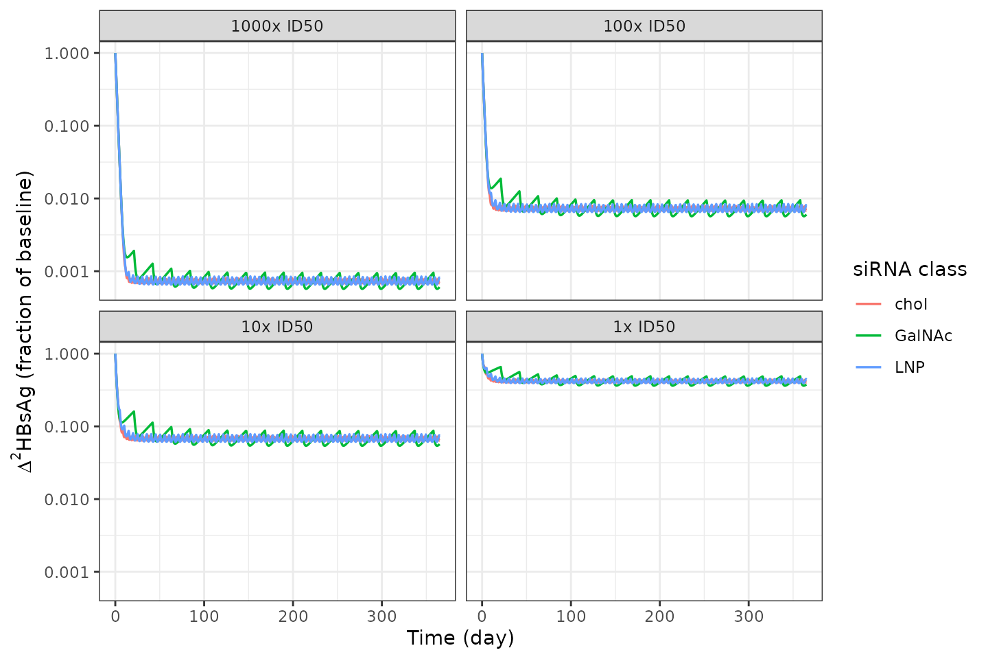

Replicates Figure 6a of Sandra 2024: deterministic multiple-dose simulations over one year, with the inter-dose interval set to each class’s biophase half-life, at 1, 10, 100 and 1000 times ID50. One representative compound per class.

Sandra 2024 also reports that the three classes reach similar log-drop and AOC levels between four weeks and one year under these equipotent regimens, and that GalNAc gives a more prolonged effect. The steady-state nadir under repeated dosing is therefore expected to be comparable across classes, in contrast to the single-dose case in Validation 5:

multiSummary <- multiDose |>
  dplyr::filter(time >= 28) |>
  dplyr::group_by(class, fold) |>
  dplyr::summarise(nadir_logdrop = -log10(min(Cc)), .groups = "drop") |>
  tidyr::pivot_wider(names_from = class, values_from = nadir_logdrop)

stopifnot(
  # "Similar LD and AOC levels between 4 weeks and 1 year": the three classes
  # sit within a factor of two of each other on log drop at every dose level,
  # whereas the single-dose gap in Validation 5 is much wider. Deterministic.
  all(
    pmax(multiSummary$GalNAc, multiSummary$LNP, multiSummary$chol) /
      pmin(multiSummary$GalNAc, multiSummary$LNP, multiSummary$chol) < 2
  )
)

multiSummary |>
  dplyr::rename("ID50-fold dose" = fold) |>
  knitr::kable(digits = 3)

ID50-fold dose	GalNAc	LNP	chol
1	0.441	0.407	0.397
10	1.267	1.213	1.197
100	2.245	2.187	2.170
1000	3.243	3.184	3.168

Validation 7: the response recovers to baseline after the biophase empties

Once the biophase compartment has drained, inhibition ends and the indirect response must relax back to its pre-treatment value of exactly 1. The relaxation rate is kdeg, so recovery is essentially complete within a few days of the biophase emptying regardless of class.

recovery <- lapply(c("GalNAc", "LNP", "chol"), function(cls) {
  column <- sirna$column[sirna$class == cls][1]
  id50I <- sirna$id50_paper[sirna$class == cls][1]
  s <- solveSingle(column, dose = 1000 * id50I, times = seq(0, 730, by = 1))
  tibble::tibble(
    class      = cls,
    nadir      = min(s$Cc),
    final      = s$Cc[nrow(s)],
    time_final = s$time[nrow(s)]
  )
})
#> ℹ omega/sigma items treated as zero: 'eta_study_lkdeg'
#> ℹ omega/sigma items treated as zero: 'eta_study_lkdeg'
#> ℹ omega/sigma items treated as zero: 'eta_study_lkdeg'
recovery <- dplyr::bind_rows(recovery)

stopifnot(
  # Deep suppression during treatment ...
  all(recovery$nadir < 0.1),
  # ... and full recovery to the corrected baseline of 1 by two years.
  max(abs(recovery$final - 1)) < 1e-4
)

recovery |>
  dplyr::select("Class" = class, "Nadir" = nadir,
                "Response at 730 days" = final) |>
  knitr::kable(digits = 6)

Class	Nadir	Response at 730 days
GalNAc	0.001551	1
LNP	0.000058	1
chol	0.008011	1

Assumptions and deviations

Simulation scope is the study-arm mean, not the individual mouse. The only random effect in the model is a between-STUDY variance on kdeg, encoded as eta_study_lkdeg per the MBMA convention. There is no between-subject variability anywhere in this model, so it cannot produce individual-animal HBsAg trajectories.
The residual is not reweighted inside the model. Sandra 2024 Eq 9 makes the residual SD expSd * CV%_ijt / sqrt(N_ijt - 1), where the CV% and the arm size are digitised properties of each published study arm. Those are properties of the fitted dataset rather than of the model, so, following the Boucher_2018_naproxen_mbma and Vargo_2014_statins_ezetimibe_mbma precedent, the model exposes only the Eq 9 sigma (expSd = 0.0342) and leaves the per-observation reweighting to downstream code. Applying expSd unscaled understates the residual badly: because Eq 1 puts CV% on the percent scale, a typical arm here (CV% about 30, n = 5) has an operative log-scale SD of 0.0342 * 30 / sqrt(4) = about 0.51, roughly fifteen times the bare value. Every simulation in this vignette is deterministic, so none of them is affected.
Between-study variability on KDE and ID50 is absent by design. Sandra 2024 Table 2 shows both collapsed to negligible values once the class effect on KDE and the siRNA-specific effect on ID50 were added, and its note records that “negligible BSV estimate values were fixed to 0”. They are omitted from ini() rather than written as ~ fixed(0), because a zero-variance diagonal makes the omega matrix singular and breaks rxSolve.
BSV kdeg is read as an omega standard deviation, not a log-normal CV. Table 3 reports 31.4% (31.39% unrounded in Table 2) and the Results text separately converts it, with a cited formula, to “a CV% of 32.31%”. There would be nothing to convert if the table already held the log-normal CV, and sqrt(exp(0.3139^2) - 1) = 0.3218 does land at about the quoted 32.3%. The ini() variance is therefore 0.3139^2 = 0.0985. The residual row cannot arbitrate this, because at 3.42% the two conventions differ in the fourth decimal place.
The delivery class is derived from the treatment indicator, not supplied. Each of the 13 siRNAs belongs to exactly one class in Sandra 2024 Table 1, so carrying separate class columns would allow a drug/class pair the paper does not contain. Set exactly one TRT_* indicator to 1; the class-specific kel follows.
The 74 + 77 combination is a single entity. Sandra 2024 fits NAG-MLP chol-siHBV-74 + 77 with its own ID50 (41.46 ng, the most potent in the analysis) rather than as a combination of two separately parameterised siRNAs. Use TRT_SIHBV74_77; do not set both TRT_SIHBV74 and TRT_SIHBV77.
Doses are absolute amounts in ng. Sandra 2024 converted published mg/kg doses using the reported mean bodyweight, assuming 20 g where a study did not report one. A model consumer must do the same conversion; passing a mg/kg number directly would misstate the potency ratio by roughly five orders of magnitude.
Route of administration and murine HBV model are not covariates. The paper made no adaptation for IV versus SC, on the grounds that SC absorption of GalNAc-siRNAs is complete and that plasma and liver kinetics are completely temporally disconnected. HDI versus AAV-HBV was tested on kdeg and neither improved the fit nor reduced the between-study variability.
Representative compounds in Figures 4 and 6. Sandra 2024 stratifies these figures by class. This vignette plots one compound per class (ALG-125755, ARB-1467, NAG-MLP chol-siHBV-74); Validation 5 uses all 13.
One published comparison does not reproduce on a class median. The Results claim that GalNAc gives the larger nadir than the other two classes “across all simulated ID50-fold dose levels” reproduces on the envelope of Figure 5 (the class maximum) but not on the class median, where GalNAc falls below LNP at 10x ID50 and above. The cause is the Hill exponent, which was estimated for only three of the thirteen compounds and dominates the nadir at doses above ID50. This is set out with the measured values under Validation 5 and is deliberately excluded from that section’s assertions rather than having the bound widened until it passed. The paper’s AOC / duration-of- response conclusions are unaffected.

Errata

Cholesterol biophase half-life, Discussion. The Discussion states “GalNAc-siRNAs show a prolonged biophase half-life of 21.1 days, compared to 5.1 days for LNP-siRNAs and 1.3 days for chol-siRNAs”. The Abstract, the Results and Table 3 all give 2.89 days for the cholesterol class, and ln(2)/0.2403 = 2.884 confirms 2.89 is the value consistent with the published KDE estimate. The Discussion’s 1.3 is a typographical error and this model uses the Table 3 value. The number 1.313 does appear in Table 3, as the Hill exponent for NAG-MLP chol-siHBV-77, which is the likely source of the slip.
BSV on kdeg, Results versus tables. The Results text quotes 32.31% where Tables 2 and 3 give 31.39% and 31.4%. These are the same quantity expressed on two conventions, as set out under Assumptions above; the small residual mismatch (32.18% recomputed versus 32.31% printed) is rounding of the omega before it was tabulated.
Study count. The Results say the final dataset included “nine placebo or vehicle-controlled non-clinical studies” while the Abstract says “Literature data from 10 studies”. Table 1 lists ten rows, two of which are the same reference (Amy C.H. Lee 2018, reference 40) contributing two separate experiments, which reconciles the two statements. The model metadata records n_studies = 9.