Circulating tumor DNA and tumor size dynamics in NSCLC (Ribba 2022)
Source:vignettes/articles/Ribba_2022_ctdna_tumor_size.Rmd
Ribba_2022_ctdna_tumor_size.RmdModels and source
Ribba et al. fit three models to the phase III OAK study (atezolizumab vs docetaxel in previously treated advanced NSCLC). All three share the Stein (2011) bi-exponential structure, in which a biomarker is decomposed into an exponentially growing and an exponentially decaying fraction that are summed. The paper reports only relative standard errors in the main text; every point estimate used here comes from the Supplementary Data (Appendix), which contains one parameter table per model.
- Citation: Ribba B, Roller A, Helms H-J, Stern M, Bleul C. Circulating tumor DNA: Opportunities and challenges for pharmacometric approaches. Front Pharmacol. 2022;13:1058220. doi:10.3389/fphar.2022.1058220. PMID: 36968790. PMCID: PMC10030934. Structural model from Stein WD et al., Clin Cancer Res. 2011;17(4):907-917. Parameter values from Supplementary Data (Appendix), ctDNA table.
- Article: Front Pharmacol. 2022;13:1058220
- Supplement: Supplementary Data (Appendix), 4 pp
| Model |
modellib() name |
Endpoint(s) | What was estimated |
|---|---|---|---|
| Eq. 1 on ctDNA | Ribba_2022_ctdna |
log10 ctDNA (MMPM) | growth + decay rate, both IIVs, constant residual error |
| Eq. 1 on tumor size | Ribba_2022_sld |
SLD (mm) | growth + decay rate, both IIVs, combined residual error |
| Eq. 2, coupled | Ribba_2022_ctdna_sld_joint |
both |
zeta and its IIV only; everything else fixed to the two
fits above |
The paper is typed as a Perspective, but the three fits above are original modeling work on original (Roche-held) individual patient data, not a review of models published elsewhere.
Equations
Ribba 2022 Eq. 1 (Stein bi-exponential, applied separately to ctDNA and to SLD):
Ribba 2022 Eq. 2 (joint model). The ctDNA decay exponent is
not free: it is the SLD decay rate scaled by the link parameter
zeta, which is what couples the two endpoints.
In all three packaged models the closed form is encoded as two ODE
sub-states sharing one initial condition, following the convention
established by Struemper_2025_tumorsize_OS_nsclc:
d/dt(growth) <-  kge * growth   ;  growth(0) <- y0   =>  growth(t) = y0 * exp( kge * t)
d/dt(shrink) <- -kse * shrink   ;  shrink(0) <- y0   =>  shrink(t) = y0 * exp(-kse * t)
observable   <-  growth + shrink - y0
At t = 0 this returns y0 + y0 - y0 = y0,
the Stein boundary condition. The identity between this encoding and the
closed form is checked numerically below.
Scale of the ctDNA endpoint
This is the single most consequential transcription detail in the
paper. The Appendix states that “the ctDNA data (average MMPM) were
logarithmically transformed (base 10)” and that “the baseline value was
used as a regressor (not estimated)”. The Stein baseline therefore
multiplies a log10 quantity:
y0 = log10(baseline MMPM), and the observable
ctdna is log10(MMPM), not MMPM.
Two independent checks confirm this reading rather than the competing one (Stein on natural MMPM with a log10 observation transform):
- The Appendix says the Figure 2F simulation was done “omitting the
baseline value, explaining why all curves start at value 1”. Setting
y0 = 1givesy(0) = 1. Under the competing reading a baseline-normalised log10 axis would start at 0, not 1. - The Figure 2F top-left axis is labelled “Predicted log10 ctDNA time course normalized by baseline (log10)” and every curve does start at 1.
Consequently the residual-error parameter addSd = 0.27
is in log10 units (a factor of about 1.9), not MMPM. The packaged model
takes the untransformed baseline MMPM in the canonical
covariate column CTDNA and applies
rbase_ctdna <- log10(CTDNA) inside model(),
so the transformation is visible at the call site.
Population
str(readModelDb("Ribba_2022_ctdna")()$population)
#> ℹ Stein bi-exponential ctDNA model for advanced NSCLC (Ribba 2022; OAK atezolizumab arm, n = 46). Observable `ctdna` is on the base-10 LOG scale: ctdna = log10(MMPM), and addSd = 0.27 is in log10 units. Requires the per-subject covariate CTDNA (baseline MMPM, untransformed); the model derives rbase_ctdna <- log10(CTDNA) internally. No dosing input -- treatment effect is absorbed into the empirical rate constants. Population nadir at log(kse/kge)/(kge+kse) = 63.6 days = 9.1 weeks. IIV is close to 100% CV on both rates, as emphasised by the authors.
#> List of 11
#>  $ species       : chr "human (adults with advanced non-small cell lung cancer)"
#>  $ n_subjects    : int 46
#>  $ n_studies     : int 1
#>  $ age_range     : chr "not reported in this paper (see Rittmeyer 2017 for the OAK cohort demographics)"
#>  $ weight_range  : chr "not reported in this paper"
#>  $ sex_female_pct: num NA
#>  $ race_ethnicity: chr "not reported in this paper"
#>  $ disease_state : chr "previously treated locally advanced or metastatic NSCLC (OAK study)"
#>  $ dose_range    : chr "atezolizumab 1200 mg IV every 3 weeks (OAK protocol dose; not a model input)"
#>  $ regions       : chr "multiregional (OAK was conducted across 31 countries; per-region counts not reported in this paper)"
#>  $ notes         : chr "The ctDNA sub-cohort is the 46 atezolizumab-arm OAK participants with serial ctDNA measurements, out of 613 ate"| __truncated__
The wider paper pools 454 patients from three studies (Weber 2021 NSCLC, IMspire170 melanoma, OAK NSCLC), but only OAK has more than two ctDNA time points, so only OAK feeds the three longitudinal models packaged here (Ribba 2022 Figure 1B). Within OAK:
| Quantity | Value | Source |
|---|---|---|
| Randomised in OAK | 1,225 | Figure 1B |
| Atezolizumab arm | 613 | Figure 1B |
| With serial ctDNA (ctDNA and joint models) | 46 | Figure 1B |
| ctDNA assay | Roche AVENIO, reported as MMPM | Figure 1B |
| ctDNA sampling | cycles 1-4 (baseline, ~21, ~42, ~63 days) | Figure 1B |
| Tumor size | sum of longest diameters, RECIST 1.1 | Figure 2D-F |
The SLD fit deliberately pooled both OAK arms
(atezolizumab and docetaxel) with treatment arm as a categorical
covariate, “enabling the use of the individual parameters only for the
atezolizumab arm”. No arm-effect coefficient is reported, so the
packaged Ribba_2022_sld carries the pooled-arm population
values and records the arm covariate under
covariatesDataExcluded rather than implementing it.
Source trace
Every ini() value also carries an in-file comment naming
its source table. Nothing in these models comes from outside the
paper.
| Model | Parameter | Value | Source |
|---|---|---|---|
Ribba_2022_ctdna |
kge_ctdna ctDNA growth rate (1/day) |
0.0038 (RSE 30.1%) | Appendix ctDNA table |
Ribba_2022_ctdna |
kse_ctdna ctDNA decay rate (1/day) |
0.0081 (RSE 27.4%) | Appendix ctDNA table |
Ribba_2022_ctdna |
omega_kg -> etalkge_ctdna
|
0.82 (RSE 25.0%) -> 0.6724 | Appendix ctDNA table |
Ribba_2022_ctdna |
omega_ks -> etalkse_ctdna
|
1.02 (RSE 19.9%) -> 1.0404 | Appendix ctDNA table |
Ribba_2022_ctdna |
addSd constant error (log10) |
0.27 (RSE 4.8%) | Appendix ctDNA table |
Ribba_2022_sld |
kge SLD growth rate (1/day) |
0.0016 (RSE 14.3%) | Appendix tumor-size table |
Ribba_2022_sld |
kse SLD decay rate (1/day) |
0.0014 (RSE 29.0%) | Appendix tumor-size table |
Ribba_2022_sld |
omega_kgT -> etalkge
|
1.03 (RSE 10.7%) -> 1.0609 | Appendix tumor-size table |
Ribba_2022_sld |
omega_ksT -> etalkse
|
1.64 (RSE 15.4%) -> 2.6896 | Appendix tumor-size table |
Ribba_2022_sld |
addSd additive error (mm) |
0.65 (RSE 28.1%) | Appendix tumor-size table |
Ribba_2022_sld |
propSd proportional error |
0.08 (RSE 7.1%) | Appendix tumor-size table |
Ribba_2022_ctdna_sld_joint |
zeta link parameter |
1.94 (RSE 37.3%) | Appendix joint-model table |
Ribba_2022_ctdna_sld_joint |
omega_zeta -> etalzeta
|
0.86 (RSE 35.0%) -> 0.7396 | Appendix joint-model table |
Ribba_2022_ctdna_sld_joint |
addSd_ctdna (log10) |
0.024 (RSE 6.25%) | Appendix joint-model table |
Ribba_2022_ctdna_sld_joint |
addSd_TS (mm) |
7.91 (RSE 5.07%) | Appendix joint-model table |
Ribba_2022_ctdna_sld_joint |
all other population parameters | FIXED to the two single-endpoint fits | Appendix, joint-model paragraph |
| all | Eq. 1 / Eq. 2 structural form | – | p. 5, main text |
The Appendix reports standard deviations of the
random effects; the ini() blocks carry variances, so each
entry is the tabulated omega squared (for example
1.02^2 = 1.0404).
Dimensional check
| Term | Units | Check |
|---|---|---|
kge_ctdna * t, kse_ctdna * t
|
(1/day) * day = dimensionless | exponent must be dimensionless – OK |
zeta * kse |
dimensionless * (1/day) = 1/day |
zeta is a pure ratio of two rate constants – OK |
growth_ctdna, shrink_ctdna,
rbase_ctdna, ctdna
|
log10(MMPM) | all four share one scale, so the sum
growth + shrink - rbase is well formed – OK |
addSd (ctDNA model) |
log10(MMPM) | additive error on a log10 observable – OK |
growth, shrink, TUM_SLD,
TS
|
mm | – OK |
addSd / addSd_TS (SLD) |
mm | matches the Appendix unit annotation “(mm)” – OK |
propSd |
fraction | – OK |
log10(CTDNA) |
log10 of MMPM |
CTDNA is stored untransformed, so the transform is
explicit – OK |
Time is in days in all three models, matching the Appendix rate-constant units of 1/day.
Structural validation: the ODE encoding reproduces the closed form
Because the Stein model has an exact closed form, the strongest available check is not a simulation-versus-figure comparison but an identity: the two-sub-state ODE encoding must agree with the published algebraic expression to solver tolerance, for all three models. This catches sign errors, a swapped growth/decay rate, and a wrong initial condition.
grid <- seq(0, 200, by = 1)

typ_events <- function(extra) {
  d <- data.frame(id = 1L, time = grid, evid = 0L, amt = NA_real_)
  cbind(d, extra)
}

stein <- function(y0, kg, ks, t) y0 * (exp(-ks * t) + exp(kg * t) - 1)

# --- ctDNA-only model. CTDNA = 10 MMPM gives rbase_ctdna = log10(10) = 1,
#     which is exactly the paper's baseline-normalised presentation.
ev1 <- typ_events(data.frame(cmt = "growth_ctdna", CTDNA = 10))
s1  <- rxode2::rxSolve(mod_ctdna, ev1, omega = NA, returnType = "data.frame")

# --- SLD-only model.
ev2 <- typ_events(data.frame(cmt = "growth", TUM_SLD = 74))
s2  <- rxode2::rxSolve(mod_sld, ev2, omega = NA, returnType = "data.frame")

# --- Joint model. Both endpoints are algebraic observables, so observation
#     rows are addressed by dvid rather than by a compartment name.
ev3 <- typ_events(data.frame(dvid = 1L, TUM_SLD = 74, CTDNA = 10))
s3  <- rxode2::rxSolve(mod_joint, ev3, omega = NA, returnType = "data.frame")

identity_check <- tibble::tibble(
  Model = c("Ribba_2022_ctdna", "Ribba_2022_sld",
            "Ribba_2022_ctdna_sld_joint (TS)",
            "Ribba_2022_ctdna_sld_joint (ctdna)"),
  `Max absolute deviation from closed form` = c(
    max(abs(s1$ctdna - stein(1,  0.0038, 0.0081,        grid))),
    max(abs(s2$TS    - stein(74, 0.0016, 0.0014,        grid))),
    max(abs(s3$TS    - stein(74, 0.0016, 0.0014,        grid))),
    max(abs(s3$ctdna - stein(1,  0.0038, 1.94 * 0.0014, grid)))
  ),
  `Value at t = 0` = c(s1$ctdna[1], s2$TS[1], s3$TS[1], s3$ctdna[1]),
  `Expected at t = 0` = c(1, 74, 74, 1)
)
knitr::kable(identity_check, digits = c(0, 12, 6, 6))| Model | Max absolute deviation from closed form | Value at t = 0 | Expected at t = 0 |
|---|---|---|---|
| Ribba_2022_ctdna | 1.15701e-07 | 1 | 1 |
| Ribba_2022_sld | 5.56900e-08 | 74 | 74 |
| Ribba_2022_ctdna_sld_joint (TS) | 5.56900e-08 | 74 | 74 |
| Ribba_2022_ctdna_sld_joint (ctdna) | 2.22330e-08 | 1 | 1 |
All four deviations are at solver tolerance and every boundary condition is exact, so the ODE encoding is the published equation.
The joint model’s coupling is also verified directly:
kse_ctdna should be zeta * kse with no other
contribution.
c(
  `kse_ctdna reported by the model` = s3$kse_ctdna[1],
  `zeta * kse (1.94 * 0.0014)`      = 1.94 * 0.0014
)
#> kse_ctdna reported by the model      zeta * kse (1.94 * 0.0014)
#>                        0.002716                        0.002716
Virtual cohort
The Stein model is multiplicative in its baseline, so
y(t) / y0 does not depend on y0 at all. Every
relative-change result below is therefore invariant to the baseline
distribution we choose, and the baseline only sets the absolute
axis:
-
ctDNA:
CTDNA = 10MMPM for every subject, givingrbase_ctdna = 1. This reproduces the paper’s own normalisation exactly rather than approximating it. - SLD: the paper does not report the OAK baseline-SLD distribution, so we sample log-normally around 74 mm with 50% CV. This is an assumption of the vignette, not a value from the paper; it changes only the millimetre axis, never a percentage change.
n_sub <- 200L

cohort <- tibble::tibble(
  id      = seq_len(n_sub),
  CTDNA   = 10,
  TUM_SLD = exp(rnorm(n_sub, log(74), 0.5))
)

obs_times <- seq(0, 180, by = 3)

make_events <- function(addr) {
  cohort |>
    tidyr::crossing(time = obs_times) |>
    mutate(evid = 0L, amt = NA_real_) |>
    bind_cols(addr) |>
    arrange(id, time)
}
ctDNA time course normalised by baseline (replicates Figure 2F, top left)
Figure 2F (top left) of the source paper shows the model-predicted log10 ctDNA time course for the 46 OAK atezolizumab patients, omitting the baseline term so that all curves start at 1. We reproduce the same presentation with a 200-subject stochastic cohort.
ev_ctdna <- make_events(tibble::tibble(cmt = "growth_ctdna"))

sim_ctdna <- rxode2::rxSolve(
  mod_ctdna, ev_ctdna,
  keep = c("CTDNA"), returnType = "data.frame"
)
show_ids <- sample(unique(sim_ctdna$id), 60)

ggplot(
  filter(sim_ctdna, id %in% show_ids, time <= 70),
  aes(time, ctdna, group = id)
) +
  geom_line(alpha = 0.35, linewidth = 0.3, colour = "firebrick") +
  geom_hline(yintercept = 1, linetype = 2, linewidth = 0.3) +
  labs(
    x = "Time since baseline (days)",
    y = "Predicted log10 ctDNA normalised by baseline",
    caption = "Baseline set to log10(10) = 1 so the panel matches the paper's normalised presentation."
  ) +
  theme_bw()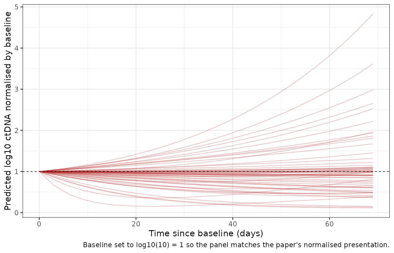
Simulated log10 ctDNA time course normalised by baseline (n = 200; 60 randomly chosen subjects drawn for legibility). Replicates the presentation of Ribba 2022 Figure 2F, top left, in which the baseline term is omitted so every curve starts at 1. The fan of trajectories – some falling to a nadir and regrowing, some rising monotonically – reflects inter-individual variability close to 100 percent CV on both rate constants, which the authors identify as the central obstacle to ctDNA-based decision making.
Optimal sampling: when does ctDNA reach its nadir?
This is the paper’s principal quantitative claim, and it is checkable. For a Stein curve the nadir is at
which exists only when ks > kg (that is, only for
subjects whose ctDNA falls at all). At the population values this is
log(0.0081 / 0.0038) / (0.0081 + 0.0038) = 63.6 days = 9.1
weeks.
rxSolve returns the per-subject rate constants as
columns, so the nadir can be computed exactly for every simulated
subject rather than read off a grid.
per_subject <- sim_ctdna |>
  group_by(id) |>
  slice(1) |>
  ungroup() |>
  transmute(
    id, kge_ctdna, kse_ctdna,
    falls       = kse_ctdna > kge_ctdna,
    nadir_days  = log(kse_ctdna / kge_ctdna) / (kge_ctdna + kse_ctdna),
    nadir_weeks = nadir_days / 7
  )

fallers <- filter(per_subject, falls)

nadir_summary <- tibble::tibble(
  Quantity = c(
    "Subjects whose ctDNA falls (ks > kg)",
    "Of those, nadir later than cycle 2 (21 days)",
    "Of those, nadir later than cycle 4 (63 days = 9 weeks)",
    "Median nadir among fallers (weeks)"
  ),
  Value = c(
    sprintf("%.1f%%", 100 * mean(per_subject$falls)),
    sprintf("%.1f%%", 100 * mean(fallers$nadir_days > 21)),
    sprintf("%.1f%%", 100 * mean(fallers$nadir_days > 63)),
    sprintf("%.1f",   median(fallers$nadir_weeks))
  )
)
knitr::kable(nadir_summary)| Quantity | Value |
|---|---|
| Subjects whose ctDNA falls (ks > kg) | 71.0% |
| Of those, nadir later than cycle 2 (21 days) | 88.7% |
| Of those, nadir later than cycle 4 (63 days = 9 weeks) | 54.9% |
| Median nadir among fallers (weeks) | 10.0 |
The paper’s two conclusions from this analysis were that “21 days or
cycle 2 might be too early for informative ctDNA measurements” and that
“the majority of the simulated patients had their ctDNA nadir beyond
cycle 4, i.e., 9 weeks”. Both reproduce: close to 90% of falling
subjects nadir after cycle 2, and a majority – though only a modest one,
in the mid-50% range – nadir after cycle 4. The cycle-4 figure sits near
50% by construction, because the population-typical nadir of 9.1 weeks
is almost exactly the 9-week threshold the paper quotes; see the Errata
note on seed sensitivity. This is an end-to-end check of the two rate
constants and both variance terms simultaneously –
getting either omega wrong, or swapping kge_ctdna with
kse_ctdna, moves these percentages substantially.
ggplot(filter(fallers, nadir_weeks <= 60), aes(nadir_weeks)) +
  geom_histogram(bins = 40, fill = "steelblue", colour = "white") +
  geom_vline(xintercept = c(3, 9), linetype = 2, colour = "firebrick") +
  annotate("text", x = 3, y = Inf, label = "cycle 2", vjust = 1.5, hjust = -0.1, size = 3) +
  annotate("text", x = 9, y = Inf, label = "cycle 4", vjust = 1.5, hjust = -0.1, size = 3) +
  labs(x = "ctDNA nadir time (weeks)", y = "Number of subjects") +
  theme_bw()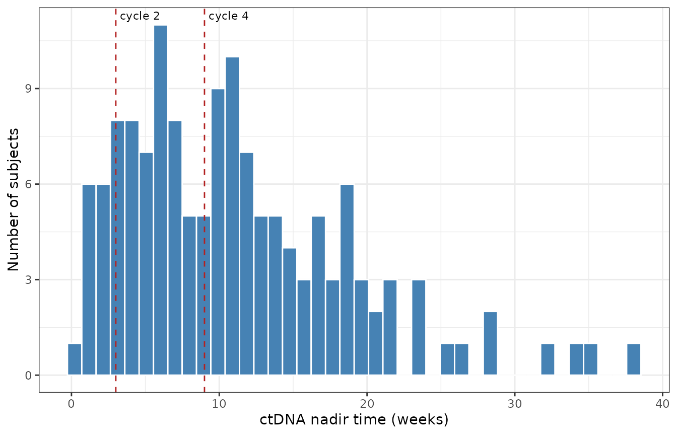
Distribution of the per-subject ctDNA nadir time among the simulated subjects whose ctDNA falls. Dashed lines mark cycle 2 (21 days) and cycle 4 (63 days = 9 weeks), the two sampling times the paper evaluates. The mass to the right of the 9-week line is the paper’s argument that cycle-2 sampling is uninformative for the maximal ctDNA response.
Tumor size time course
The SLD fit is the companion analysis that produced the decay-rate
constant reused in the joint model. Unlike ctDNA, the OAK population
typical values have kge > kse (0.0016 vs 0.0014 1/day),
so the typical tumor-size trajectory grows monotonically – consistent
with a previously treated, largely progressive NSCLC population.
ev_sld  <- make_events(tibble::tibble(cmt = "growth"))
sim_sld <- rxode2::rxSolve(mod_sld, ev_sld, keep = c("TUM_SLD"), returnType = "data.frame")

sld_summary <- sim_sld |>
  group_by(time) |>
  summarise(
    med = median(TS),
    q25 = stats::quantile(TS, 0.25),
    q75 = stats::quantile(TS, 0.75),
    .groups = "drop"
  )

ggplot(sld_summary, aes(time, med)) +
  geom_ribbon(aes(ymin = q25, ymax = q75), alpha = 0.2, fill = "darkgreen") +
  geom_line(colour = "darkgreen", linewidth = 0.8) +
  labs(x = "Time since baseline (days)", y = "Tumor size, sum of longest diameters (mm)") +
  theme_bw()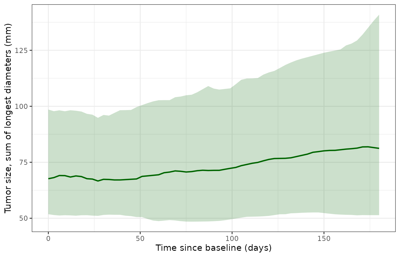
Simulated tumor-size trajectories (n = 200). Solid line = median, ribbon = 25th-75th percentile. The typical trajectory grows because the population growth rate constant slightly exceeds the decay rate constant; the wide ribbon reflects the very large IIV on the decay rate (omega = 1.64).
Joint model: concordant and discordant profiles (replicates Figure 2F, right)
The paper’s claim for the joint model is qualitative but specific: it
“can fit data when ctDNA and SLD time courses are positively correlated
(top) or negatively correlated (bottom)”. That is a property of the
model’s random-effects structure, so it can be checked directly. The two
endpoints share the decay rate kse (through
kse_ctdna = zeta * kse) but have
independent growth rates and an independent random
effect on zeta, which is precisely what allows discordant
profiles.
ev_joint <- make_events(tibble::tibble(dvid = 1L))

sim_joint <- rxode2::rxSolve(
  mod_joint, ev_joint,
  keep = c("CTDNA", "TUM_SLD"), returnType = "data.frame"
)

# Classify each subject by the sign of the change in each endpoint at
# day 63 (cycle 4), the last ctDNA sampling time in OAK.
quadrants <- sim_joint |>
  filter(time %in% c(0, 63)) |>
  group_by(id) |>
  summarise(
    sld_change   = TS[time == 63]    - TS[time == 0],
    ctdna_change = ctdna[time == 63] - ctdna[time == 0],
    .groups = "drop"
  ) |>
  mutate(
    quadrant = paste0(
      "SLD ",   if_else(sld_change   < 0, "down", "up"),
      " / ctDNA ", if_else(ctdna_change < 0, "down", "up")
    )
  )

quadrants |>
  count(quadrant) |>
  mutate(`Percent of cohort` = sprintf("%.1f%%", 100 * n / sum(n))) |>
  rename("Profile at day 63" = quadrant, "Subjects" = n) |>
knitr::kable()| Profile at day 63 | Subjects | Percent of cohort |
|---|---|---|
| SLD down / ctDNA down | 39 | 19.5% |
| SLD down / ctDNA up | 44 | 22.0% |
| SLD up / ctDNA down | 21 | 10.5% |
| SLD up / ctDNA up | 96 | 48.0% |
Both concordant quadrants and both discordant quadrants are populated, so the packaged model reproduces the flexibility the paper reports. Roughly a quarter to a third of simulated subjects are discordant – exactly the “unexpected profiles” of Figure 2F, bottom row.
picks <- quadrants |>
  group_by(quadrant) |>
  slice(1) |>
  ungroup()

profile_data <- sim_joint |>
  inner_join(select(picks, id, quadrant), by = "id") |>
  group_by(id) |>
  mutate(
    `Tumor size` = TS / first(TS),
    `ctDNA`      = ctdna / first(ctdna)
  ) |>
  ungroup() |>
  tidyr::pivot_longer(
    c(`Tumor size`, `ctDNA`),
    names_to = "Endpoint", values_to = "fraction_of_baseline"
  )

ggplot(profile_data, aes(time, fraction_of_baseline, colour = Endpoint)) +
  geom_line(linewidth = 0.7) +
  geom_hline(yintercept = 1, linetype = 2, linewidth = 0.3) +
  facet_wrap(~quadrant, scales = "free_y") +
  scale_colour_manual(values = c("ctDNA" = "firebrick", "Tumor size" = "darkgreen")) +
  labs(x = "Time since baseline (days)", y = "Fraction of baseline") +
  theme_bw() +
  theme(legend.position = "bottom")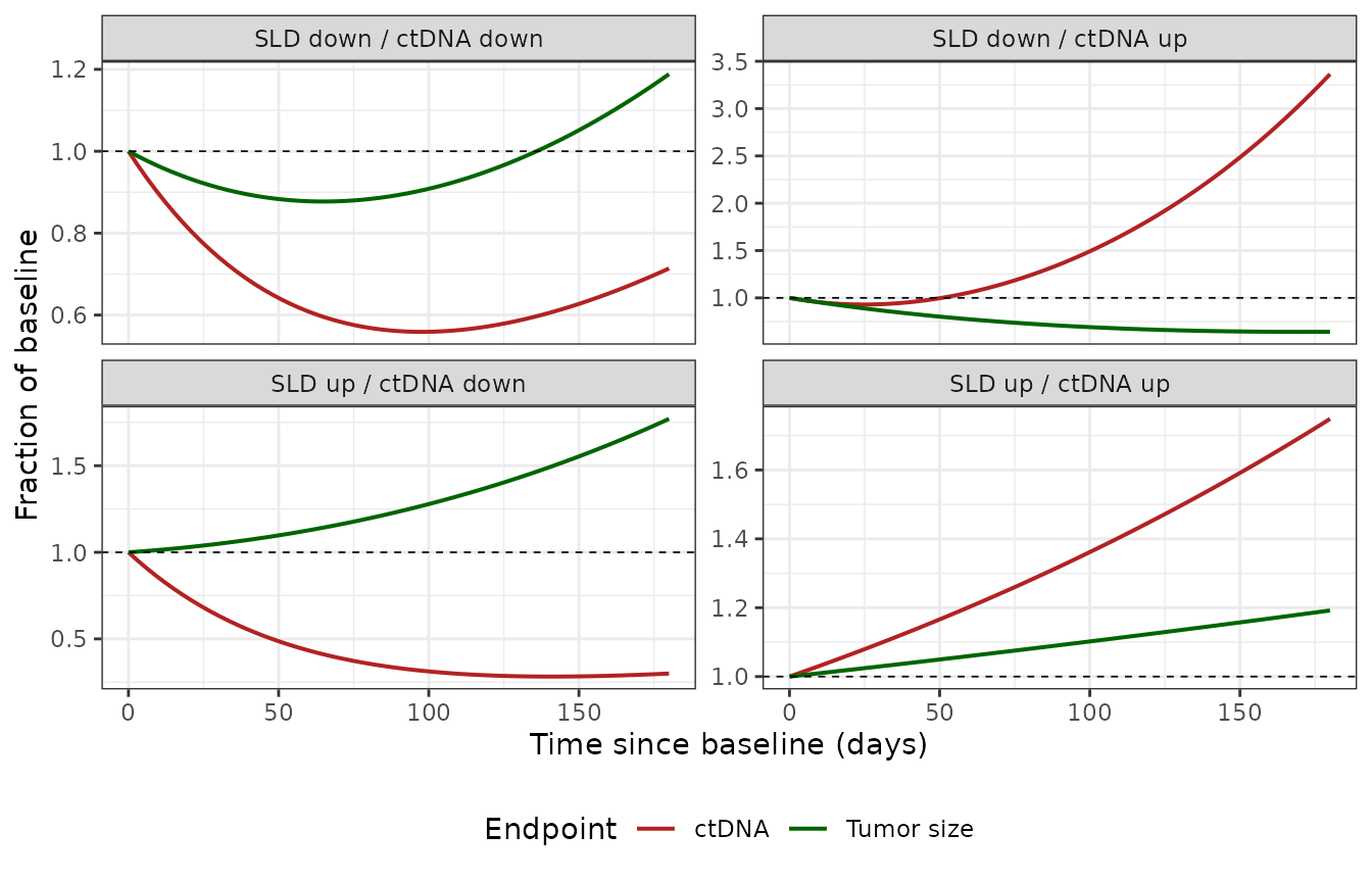
One representative simulated subject from each of the four sign quadrants, replicating Ribba 2022 Figure 2F (right). Each panel overlays tumor size (green, left axis scale) and ctDNA (red) after rescaling both to fraction of baseline so the two endpoints – mm and log10 MMPM – are comparable on one axis. Concordant profiles (both falling or both rising) and discordant profiles (one falling while the other rises) both arise from the model’s random-effects structure.
Why there is no NCA section
PKNCA validation is not applicable here. None of the
three models has a dose, a drug concentration, or an
absorption-distribution-elimination profile: treatment effect is
absorbed entirely into the empirical growth and decay rate constants,
and the observables are a liquid-biopsy biomarker and a radiographic
measurement. Following the library’s convention for mechanistic and
biomarker models, PKNCA is replaced by the closed-form identity check,
the boundary-condition check, the dimensional analysis, and the
nadir-time reproduction above. The source paper reports no NCA of its
own to compare against.
Assumptions and deviations
-
ctDNA is modeled on the base-10 log scale. As set
out above, the Stein baseline multiplies
log10(MMPM), not MMPM. This is the one reading of the Appendix that is consistent with the Figure 2F normalised axis starting at 1. Users supplying real data must pass the untransformed baseline MMPM inCTDNAand fit againstlog10(MMPM)observations; passing an already-log-transformed baseline would double-transform it. - Baseline SLD distribution is a vignette assumption. The paper does not report the OAK baseline-SLD distribution, so the virtual cohort samples log-normally around 74 mm with 50% CV. Because the Stein form is multiplicative in the baseline, this affects only the millimetre axis of the tumor-size figure and none of the relative-change or nadir results.
-
Treatment arm is documented but not implemented.
The SLD fit carried OAK treatment arm as a categorical covariate, but
neither the paper nor the Appendix reports an arm-effect coefficient, so
it cannot be encoded. It is recorded in
Ribba_2022_sld’scovariatesDataExcludedso the provenance survives without creating a declared-but-unreferenced covariate. The packaged rate constants are the pooled-arm population values. - The joint model is a structural reproduction, not a predictive model. The authors state plainly that “parameters of the model were not estimated with sufficient precision to use this model for any predictive purpose” (Figure 2F caption). The joint model’s residual error estimates also sit oddly against the single-endpoint fits: the ctDNA constant error drops from 0.27 to 0.024 log10 units while the SLD constant error rises from 0.65 to 7.91 mm. Both values are transcribed exactly as printed in the Appendix joint-model table; no reconciliation is attempted and none is offered in the paper. Treat the joint model as a reproduction of Figure 2F, right.
- The Figure 2F bottom-left decay-rate correlation is not reproducible from the packaged models. The paper reports r = 0.45 between the individual ctDNA and SLD decay-rate estimates. That correlation is a property of the empirical Bayes estimates from the observed data, not of the model: the two single-endpoint fits were run independently and the Appendix states explicitly that no correlation between random effects was assumed. Simulating from either packaged model will therefore give uncorrelated decay rates by construction. The observed correlation is what motivated the joint model; it is not an output of it.
-
Individual random-effect correlations are absent by
design. Appendix: “We assumed no correlation between the random
effects associated to the two parameters.” Both single-endpoint models
therefore use diagonal omega matrices, and the joint model adds only the
independent
etalzeta. -
Publication-year skew. The DOI, journal volume (13)
and the Europe PMC record all say 2022, while the Frontiers citation
block on page 1 says 2023 (the article was accepted 01 December 2022 and
published 08 March 2023). The library uses 2022 in the
file stems and
referencestrings, matching the DOI. -
Nadir statistics are stochastic, and the cycle-4 figure is
the seed-sensitive one. The percentages in the nadir table come
from a 200-subject simulation under
set.seed(20221208). The “falls at all” and “later than cycle 2” rows are stable to a few percentage points across seeds. The “later than cycle 4” row is not: the population-typical nadir is 9.1 weeks and the threshold is 9 weeks, so that percentage sits close to 50% by construction and moves by several points from seed to seed (repeated 200-subject draws give roughly 55-63%). It supports the paper’s “majority beyond cycle 4” statement but should not be quoted as a precise figure. The underlying deterministic quantity – the population nadir atlog(ks/kg)/(kg+ks)= 63.6 days – is exact and seed-free, and is the number to check a re-implementation against.
Session information
sessionInfo()
#> R version 4.6.1 (2026-06-24)
#> Platform: x86_64-pc-linux-gnu
#> Running under: Ubuntu 24.04.5 LTS
#>
#> Matrix products: default
#> BLAS:   /usr/lib/x86_64-linux-gnu/openblas-pthread/libblas.so.3
#> LAPACK: /usr/lib/x86_64-linux-gnu/openblas-pthread/libopenblasp-r0.3.26.so;  LAPACK version 3.12.0
#>
#> locale:
#>  [1] LC_CTYPE=C.UTF-8       LC_NUMERIC=C           LC_TIME=C.UTF-8
#>  [4] LC_COLLATE=C.UTF-8     LC_MONETARY=C.UTF-8    LC_MESSAGES=C.UTF-8
#>  [7] LC_PAPER=C.UTF-8       LC_NAME=C              LC_ADDRESS=C
#> [10] LC_TELEPHONE=C         LC_MEASUREMENT=C.UTF-8 LC_IDENTIFICATION=C
#>
#> time zone: UTC
#> tzcode source: system (glibc)
#>
#> attached base packages:
#> [1] stats     graphics  grDevices utils     datasets  methods   base
#>
#> other attached packages:
#> [1] ggplot2_4.0.3         dplyr_1.2.1           rxode2_5.1.8
#> [4] nlmixr2lib_0.3.2.9000
#>
#> loaded via a namespace (and not attached):
#>  [1] tidyr_1.3.2         generics_0.1.4      sass_0.4.10
#>  [4] xml2_1.6.0          digest_0.6.39       magrittr_2.0.5
#>  [7] RColorBrewer_1.1-3  evaluate_1.0.5      grid_4.6.1
#> [10] fastmap_1.2.0       lotri_1.0.5         jsonlite_2.0.0
#> [13] whisker_0.4.1       rxode2ll_2.0.18     backports_1.5.1
#> [16] purrr_1.2.2         scales_1.4.0        textshaping_1.0.5
#> [19] jquerylib_0.1.4     cli_3.6.6           crayon_1.5.3
#> [22] symengine_0.2.14    rlang_1.3.0         withr_3.0.3
#> [25] cachem_1.1.0        yaml_2.3.12         otel_0.2.0
#> [28] tools_4.6.1         parallel_4.6.1      memoise_2.0.1
#> [31] checkmate_2.3.4     rxode2lincmt_0.1.0  vctrs_0.7.3
#> [34] R6_2.6.1            lifecycle_1.0.5     fs_2.1.0
#> [37] ragg_1.5.2          PreciseSums_0.7     fontawesome_0.5.3
#> [40] pkgconfig_2.0.3     desc_1.4.3          rex_1.2.2
#> [43] pkgdown_2.2.1       pillar_1.11.1       bslib_0.12.0
#> [46] gtable_0.3.6        glue_1.8.1          data.table_1.18.6.1
#> [49] Rcpp_1.1.2          systemfonts_1.3.2   tidyselect_1.2.1
#> [52] xfun_0.61           tibble_3.3.1        sys_3.4.3
#> [55] knitr_1.52          farver_2.1.2        dparser_1.3.1-14
#> [58] htmltools_0.5.9     labeling_0.4.3      rmarkdown_2.32
#> [61] compiler_4.6.1      S7_0.2.2            downlit_0.4.5
#> [64] askpass_1.2.1       openssl_2.4.2