Doxorubicin + dexrazoxane cardiotoxicity in AC16 cardiomyocytes (Mody 2023)
Source:vignettes/articles/Mody_2023_doxorubicin_dexrazoxane.Rmd
Mody_2023_doxorubicin_dexrazoxane.RmdModel and source
- Citation: Mody H, Vaidya TR, Ait-Oudhia S (2023). In vitro to clinical translational pharmacokinetic/pharmacodynamic modeling of doxorubicin (DOX) and dexrazoxane (DEX) interactions: Safety assessment and optimization. Scientific Reports 13:3100. doi:10.1038/s41598-023-29964-4.
- Description: In vitro (AC16 immortalized human cardiomyocyte cell line) toxicodynamic (TD) model of doxorubicin (DOX) induced cardiotoxicity and dexrazoxane (DEX) cardioprotection, linked to clinical human pharmacokinetics for the in vitro to in vivo translation of drug-drug interaction and Q3W / Q1W dosing-regimen optimization. Clinical DOX PK is a 3-compartment mammillary model with linear elimination and 15-min IV infusion (parameters from Kontny et al. 2013, ref [30], reproduced inline in Mody 2023 Table 2 for a 1.8 m^2 body surface area typical subject). Clinical DEX PK is a 2-compartment mammillary model with linear elimination and 15-min IV infusion, originally fitted to phase 1 data reported by Earhart et al. 1982 Cancer Res 42(12):5255-61 (Mody 2023 Table 2). The TD model on AC16 has (1) an exponential-growth baseline for the untreated cell viability R, (2) a linear DOX growth-inhibition slope S_DOX on kg, (3) a linear DEX growth-inhibition slope S_DEX on kg, (4) a Hill (capacity-limited) DOX stimulation-of-death signal K_DOX = Kmax * CDOX / (KC50 + CDOX) delayed through three transit compartments K1..K3 with rate 1/tau_DOX, and (5) a Hill (capacity-limited) DEX inhibition of the DOX-death signal K_DEX = Imax * CDEX / (IC50 + CDEX). The DEX inhibition enters the transit-chain source term as a subtraction on Kmax (see Assumptions and deviations in the vignette). No IIV or residual error is fitted (Table 1 reports %RSE on point estimates only); an arbitrary 10% CV IIV is added at simulation time per the paper’s Methods. Placeholder additive residual SDs are encoded as fixed() so the model parses cleanly.
- Article: https://doi.org/10.1038/s41598-023-29964-4
Population
Mody 2023 is a translational in vitro to in vivo (IVIVT) PK / toxicodynamic (TD) modeling study of doxorubicin (DOX) induced cardiotoxicity (DIC) and dexrazoxane (DEX) cardioprotection. The TD sub-model (paper Table 1) is fit to a single in vitro experiment on AC16 immortalized adult human ventricular cardiomyocytes (Millipore Sigma-EMD, derived from primary human ventricular myocytes) seeded at 10x10^3 cells / well (100 uL) of a 96-well plate. Three exposure groups were tested over a 72 h time course with cell viability read by CCK-8 colorimetric assay at 0, 12, 24, 48, 72 h: DOX 0.5-10 uM single agent, DEX 5-100 uM single agent, and combination 0.5 uM DOX + 5-100 uM DEX.
The clinical PK sub-model (paper Table 2) is used to drive the TD sub-model in vivo. DOX PK is a 3-compartment mammillary structure with parameter values reproduced by Mody 2023 from Kontny NE et al. 2013 (paper ref [30]) for a typical adult with body-surface-area 1.8 m^2. DEX PK is a 2-compartment mammillary structure originally fit by Mody 2023 to phase 1 data reported by Earhart RH et al. 1982 (paper ref [29]). The Methods section introduces an arbitrary 10% CV inter-individual variability (IIV) on TD parameters for the 500-subject simulation cohort; the packaged model carries no fitted etas (the paper reports only per-parameter % relative standard errors from the Monolix fit).
The same information is available programmatically via
readModelDb("Mody_2023_doxorubicin_dexrazoxane")$population.
Source trace
The per-parameter origin is recorded as an in-file comment next to
each ini() entry in
inst/modeldb/therapeuticArea/oncology/Mody_2023_doxorubicin_dexrazoxane.R.
The table below collects the parameter and equation provenance in one
place.
| Equation / parameter | Value | Source location |
|---|---|---|
lcl (DOX CL, L/h/1.8 m^2) |
log(53.3) | Mody 2023 Table 2 top |
lvc (DOX Vc, L/1.8 m^2) |
log(17.7) | Mody 2023 Table 2 top |
lq (DOX Q2, L/h/1.8 m^2) |
log(58.7) | Mody 2023 Table 2 top |
lvp (DOX Vp, L/1.8 m^2) |
log(1830) | Mody 2023 Table 2 top |
lq2 (DOX Q3, L/h/1.8 m^2) |
log(21.8) | Mody 2023 Table 2 top |
lvp2 (DOX Vp2, L/1.8 m^2) |
log(71.6) | Mody 2023 Table 2 top |
lcl_dex (DEX CL = kel * V, L/h) |
log(14.6) | Mody 2023 Table 2 bottom (kel = 1/h, V = 14.6 L) |
lvc_dex (DEX Vc, L) |
log(14.6) | Mody 2023 Table 2 bottom (V = 14.6 L) |
lq_dex (DEX Q = k12 * V, L/h) |
log(14.6) | Mody 2023 Table 2 bottom (k12 = 1/h) |
lvp_dex (DEX Vp = V * k12 / k21, L) |
log(14.6) | Mody 2023 Table 2 bottom (k12 = k21 = 1/h) |
lkg (AC16 growth rate, 1/h) |
log(0.0115) | Mody 2023 Table 1 |
lr0 (AC16 baseline viability, %) |
log(101) | Mody 2023 Table 1 |
lsdex (S_DEX growth inhibition slope, 1/uM) |
log(0.00968) | Mody 2023 Table 1 |
lsdox (S_DOX growth inhibition slope, 1/uM) |
log(0.167) | Mody 2023 Table 1 |
lemax (Kmax,DOX stimulation of death, 1/h) |
log(0.0697) | Mody 2023 Table 1 |
lec50 (KC50,DOX for half-maximal death, uM) |
log(0.107) | Mody 2023 Table 1 |
lktr (1/tau_DOX transit rate, 1/h) |
log(0.126) | Mody 2023 Table 1 |
limax_dex (Imax,DEXi DEX inhibition of DOX death,
1/h) |
log(0.0625) | Mody 2023 Table 1 |
lic50_dex (IC50,DEXi DEX half-max inhibition, uM) |
log(39) | Mody 2023 Table 1 |
lconv_dox (DOX mg/L to uM, FIXED) |
log(1.8397) | PubChem CID 31703 (DOX free base MW 543.52 g/mol) |
lconv_dex (DEX mg/L to uM, FIXED) |
log(3.7275) | PubChem CID 71384 (DEX free base MW 268.27 g/mol) |
| DOX PK ODEs (3-compartment mammillary IV) | – | Mody 2023 Figure 3 (Left top) + Table 2 top |
| DEX PK ODEs (2-compartment mammillary IV) | – | Mody 2023 Eq for DEX PK + Figure 3 (Left bottom) |
| AC16 growth Eq: dR/dt = kg * R * (1 - S_DOX * CDOX) | ||
| * (1 - S_DEX * CDEX) - transit3 * R | – | Mody 2023 Eq 3 (control), Eq 4e (S_DOX), Eq 5 (S_DEX), Eq 6a-f (combo) |
| DOX stimulation-of-death Hill Eq | – | Mody 2023 Eq 4a-c (K_DOX = Kmax * CDOX / (KC50 + CDOX)) |
| DEX inhibition-of-DOX-death Hill Eq | – | Mody 2023 Eq 6a-f (K_DEX = Imax * CDEX / (IC50 + CDEX)) |
| 3-transit-compartment delay chain | – | Mody 2023 text (“three transit compartments … 1/tau_DOX”) |
The residual error parameters (addSd,
addSd_dex, addSd_viability) are
maintainer-chosen placeholders – Mody 2023 does not tabulate a residual
SD – and are flagged with fixed() so they do not contribute
false precision.
Simulation setup
The packaged model is solved deterministically (paper reports no
fitted IIV; the zeroRe() call zeroes the placeholder
residual errors so that the typical trajectory is recovered). Doses are
applied as 15-min IV infusions into central (DOX) and
central_dex (DEX); observations are scheduled per-output
(Cc, Cc_dex, viability) following
the multi-output cmt = <output-name> idiom.
mod         <- rxode2::rxode(readModelDb("Mody_2023_doxorubicin_dexrazoxane"))
mod_typical <- rxode2::zeroRe(mod)
#> Warning: No omega parameters in the model

# For a typical adult with BSA 1.8 m^2 (Mody 2023 Methods; paper Table 2
# CL / V / Q values are per-1.8 m^2)
bsa <- 1.8

# Convert mg/m^2 to mg for a 1.8 m^2 subject
mgpm2_to_mg <- function(dose_per_m2) dose_per_m2 * bsa
In vitro degradation-driven TD simulation (Figures 2A-C)
Figures 2A-C are in vitro experiments where DOX and DEX bath
concentrations degrade in cell culture media over time with the paper’s
first-order rate constants kdeg_DOX = 0.022 /h and
kdeg_DEX = 0.054 /h (Results paragraph 1, Figure 2A). These
rate constants describe the media-degradation kinetics and are used only
in vitro; the packaged translational model uses clinical PK to drive
CDOX / CDEX in vivo, so this in vitro validation uses a small auxiliary
rxode2 model that implements Eqs 1 and 2 (degradation) coupled to the TD
equations from Table 1.
# Auxiliary in vitro model: degradation-driven bath concentrations + the
# same TD structure that lives in the clinical model. Parameter values
# are transcribed from Mody 2023 Table 1 and the paper's Results text
# (kdeg values only reported in prose).
invitro_mod <- rxode2::rxode2({
  kdeg_dox  <- 0.022    # Mody 2023 Results par 1 (Fig 2A caption)
  kdeg_dex  <- 0.054    # Mody 2023 Results par 1 (Fig 2A caption)
  kg        <- 0.0115   # Table 1
  r0_val    <- 101      # Table 1
  s_dex     <- 0.00968  # Table 1
  s_dox     <- 0.167    # Table 1
  emax      <- 0.0697   # Table 1
  ec50      <- 0.107    # Table 1
  ktr       <- 0.126    # Table 1
  imax_dex  <- 0.0625   # Table 1
  ic50_dex  <- 39       # Table 1

  d/dt(bath_dox) <- -kdeg_dox * bath_dox    # Eq 1
  d/dt(bath_dex) <- -kdeg_dex * bath_dex    # Eq 2

  k_dex_inhib <- imax_dex * bath_dex / (ic50_dex + bath_dex)
  k_dox_stim  <- (emax - k_dex_inhib) * bath_dox / (ec50 + bath_dox)

  d/dt(transit1) <- ktr * (k_dox_stim - transit1)
  d/dt(transit2) <- ktr * (transit1   - transit2)
  d/dt(transit3) <- ktr * (transit2   - transit3)

  d/dt(viab) <- kg * viab * (1 - s_dox * bath_dox) * (1 - s_dex * bath_dex) -
                transit3 * viab

  viab(0) <- r0_val
})
Figure 2A – Degradation kinetics of DOX and DEX in cell culture media
Simulate bath concentrations of DOX at 0.5, 1, 5, 10 uM and DEX at 5,
25, 50, 100 uM over 72 h. Each starts at its nominal dose and decays
with the respective kdeg.
dox_levels <- c(0.5, 1, 5, 10)
dex_levels <- c(5, 25, 50, 100)

# DOX degradation curves
sim_dox_deg <- purrr::map_dfr(dox_levels, function(cd) {
  ev <- rxode2::et(amt = cd, cmt = "bath_dox", time = 0) |>
    rxode2::et(seq(0, 72, by = 1), cmt = "bath_dox")
  as.data.frame(rxode2::rxSolve(invitro_mod, ev)) |>
    dplyr::mutate(init_conc = cd, drug = "DOX")
})

sim_dex_deg <- purrr::map_dfr(dex_levels, function(cd) {
  ev <- rxode2::et(amt = cd, cmt = "bath_dex", time = 0) |>
    rxode2::et(seq(0, 72, by = 1), cmt = "bath_dex")
  as.data.frame(rxode2::rxSolve(invitro_mod, ev)) |>
    dplyr::mutate(init_conc = cd, drug = "DEX")
})

deg_data <- dplyr::bind_rows(
  sim_dox_deg |> dplyr::transmute(time, init_conc, drug, conc = bath_dox),
  sim_dex_deg |> dplyr::transmute(time, init_conc, drug, conc = bath_dex)
)

ggplot(deg_data, aes(x = time, y = conc, color = factor(init_conc))) +
  geom_line(linewidth = 0.9) +
  facet_wrap(~drug, scales = "free_y") +
  scale_x_continuous("Time (h)", breaks = c(0, 12, 24, 48, 72)) +
  scale_y_continuous("Concentration (uM)") +
  theme_bw() +
  labs(color = "Initial (uM)",
       title = "DOX and DEX degradation kinetics in cell culture media")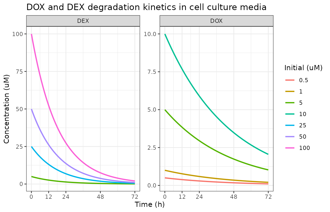
Replicates Mody 2023 Figure 2A: degradation of DOX (top curves) and DEX (bottom set) in cell culture media over 72 h.
Figure 2B – Single-agent DOX and DEX effects on AC16 cell viability
The single-agent TD experiments expose AC16 to a range of DOX (0.5 to 10 uM) or DEX (5 to 100 uM) initial bath concentrations over 72 h. DOX suppresses cell viability in a dose-dependent, delayed manner; DEX produces only slight growth inhibition.
sim_dox_only <- purrr::map_dfr(dox_levels, function(cd) {
  ev <- rxode2::et(amt = cd, cmt = "bath_dox", time = 0) |>
    rxode2::et(seq(0, 72, by = 1), cmt = "bath_dox")
  as.data.frame(rxode2::rxSolve(invitro_mod, ev)) |>
    dplyr::mutate(init_conc = cd, drug = "DOX")
})

sim_dex_only <- purrr::map_dfr(dex_levels, function(cd) {
  ev <- rxode2::et(amt = cd, cmt = "bath_dex", time = 0) |>
    rxode2::et(seq(0, 72, by = 1), cmt = "bath_dex")
  as.data.frame(rxode2::rxSolve(invitro_mod, ev)) |>
    dplyr::mutate(init_conc = cd, drug = "DEX")
})

viab_data <- dplyr::bind_rows(sim_dox_only, sim_dex_only) |>
  dplyr::select(time, init_conc, drug, viab)

ggplot(viab_data, aes(x = time, y = viab, color = factor(init_conc))) +
  geom_line(linewidth = 0.9) +
  facet_wrap(~drug) +
  geom_hline(yintercept = 101, linetype = "dashed", color = "grey60") +
  scale_x_continuous("Time (h)", breaks = c(0, 12, 24, 48, 72)) +
  scale_y_continuous("AC16 cell viability (%)") +
  theme_bw() +
  labs(color = "Initial (uM)",
       title = "Single-agent DOX and DEX effects on AC16 cell viability")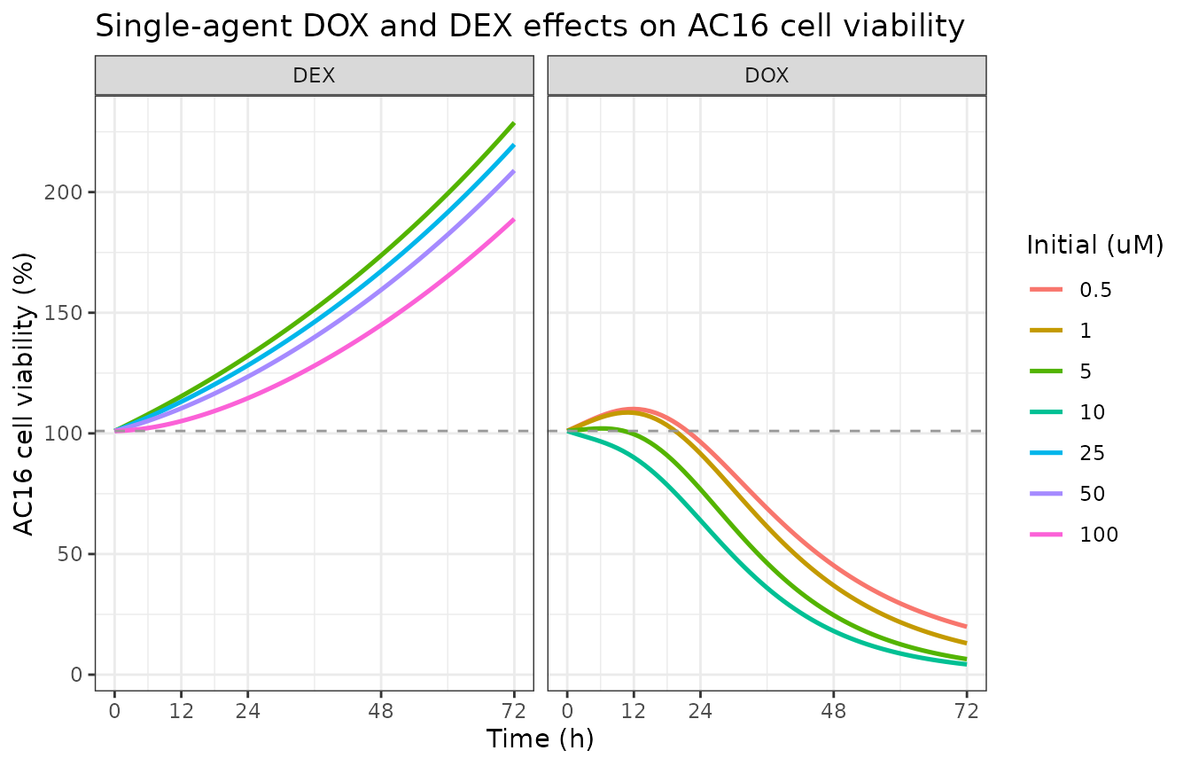
Replicates Mody 2023 Figure 2B: single-agent DOX (top row) and DEX (bottom row) effects on AC16 cell viability over 72 h.
Figure 2C – Combination DOX + DEX effects on AC16 cell viability
The combination experiments fix DOX at 0.5 uM and vary DEX from 0 to 100 uM. DEX provides dose-dependent cardioprotection: increasing DEX partially offsets the DOX-induced kill.
combo_dex <- c(0, 5, 25, 50, 100)
sim_combo <- purrr::map_dfr(combo_dex, function(cx) {
  ev <- rxode2::et(amt = 0.5, cmt = "bath_dox", time = 0) |>
    rxode2::et(amt = cx,  cmt = "bath_dex", time = 0) |>
    rxode2::et(seq(0, 72, by = 1), cmt = "viab")
  as.data.frame(rxode2::rxSolve(invitro_mod, ev)) |>
    dplyr::mutate(dex_init = cx)
})

ggplot(sim_combo, aes(x = time, y = viab, color = factor(dex_init))) +
  geom_line(linewidth = 0.9) +
  scale_x_continuous("Time (h)", breaks = c(0, 12, 24, 48, 72)) +
  scale_y_continuous("AC16 cell viability (%)") +
  theme_bw() +
  labs(color = "DEX (uM)",
       title = "Combination DOX (0.5 uM) + DEX effects on AC16 cell viability",
       subtitle = "Increasing DEX progressively protects against DOX-induced kill")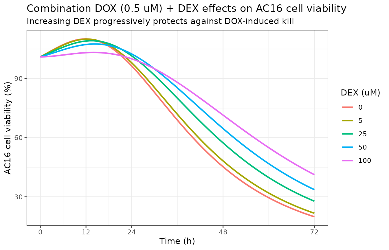
Replicates Mody 2023 Figure 2C: combination DOX (0.5 uM) + DEX (0 to 100 uM) effects on AC16 cell viability over 72 h.
Figures 4A-D – Clinical PK simulations for DOX and DEX
Figures 4A-D show simulated plasma PK for DOX at 20 to 60 mg/m^2 (Q3W IV 15-min infusion, three cycles over 9 weeks) and DEX at ratios of 1:1, 5:1, 10:1, 20:1, and 50:1 relative to 50 mg/m^2 DOX. The clinical PK model from Table 2 drives these predictions.
dox_mgm2 <- c(20, 30, 40, 50, 60)
dex_ratios <- c(1, 5, 10, 20, 50)
dox_dose_mg <- mgpm2_to_mg(dox_mgm2)          # 36, 54, 72, 90, 108 mg for BSA=1.8

# 3-cycle Q3W: doses at 0, 3, 6 weeks (in hours: 0, 504, 1008)
q3w_times <- c(0, 3, 6) * 7 * 24              # 0, 504, 1008 h

# Observation grid: dense for the first 24 h after each dose, sparser
# between doses. Total window 0 to 9 weeks + 1 week wash = 1680 h.
obs_dense_by_dose <- function(dt) {
  seq(dt, dt + 24, by = 0.25)                 # 15-min sampling for first day
}
obs_grid <- sort(unique(c(
  unlist(lapply(q3w_times, obs_dense_by_dose)),
  seq(0, 1680, by = 6)
)))
Figure 4A - DOX plasma PK over 3 cycles
sim_dox_pk <- purrr::map_dfr(seq_along(dox_mgm2), function(i) {
  dose_amt  <- dox_dose_mg[i]
  rate_amt  <- dose_amt / 0.25   # 15-min = 0.25 h infusion
  ev <- purrr::reduce(q3w_times, function(acc, t0) {
    rxode2::et(acc, amt = dose_amt, rate = rate_amt, cmt = "central", time = t0)
  }, .init = rxode2::et()) |>
    rxode2::et(obs_grid, cmt = "Cc")
  as.data.frame(rxode2::rxSolve(mod_typical, ev, useLinCmt = FALSE)) |>
    dplyr::mutate(dose_mgm2 = dox_mgm2[i])
})

ggplot(sim_dox_pk, aes(x = time / 24 / 7, y = Cc, color = factor(dose_mgm2))) +
  geom_line(linewidth = 0.7) +
  scale_x_continuous("Time (weeks)", breaks = 0:10) +
  scale_y_log10("DOX plasma concentration (mg/L)",
                labels = scales::label_number()) +
  theme_bw() +
  labs(color = "DOX dose (mg/m^2)",
       title = "DOX plasma PK over three Q3W dosing cycles")
#> Warning in scale_y_log10("DOX plasma concentration (mg/L)", labels =
#> scales::label_number()): log-10 transformation introduced infinite values.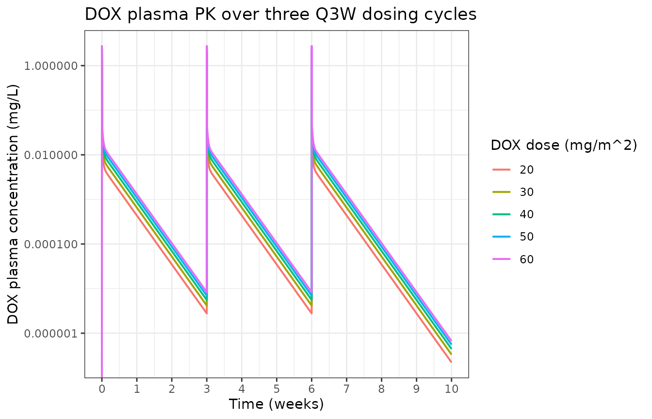
Replicates Mody 2023 Figure 4A: DOX plasma concentration over three Q3W dosing cycles at 20, 30, 40, 50, 60 mg/m^2.
Figure 4B - DOX plasma PK over a single cycle
ggplot(dplyr::filter(sim_dox_pk, time <= 24), aes(x = time, y = Cc, color = factor(dose_mgm2))) +
  geom_line(linewidth = 0.8) +
  scale_x_continuous("Time (h)", breaks = c(0, 0.25, 1, 3, 6, 12, 24)) +
  scale_y_log10("DOX plasma concentration (mg/L)",
                labels = scales::label_number()) +
  theme_bw() +
  labs(color = "DOX dose (mg/m^2)",
       title = "DOX plasma PK over one Q3W dosing cycle (first 24 h)")
#> Warning in scale_y_log10("DOX plasma concentration (mg/L)", labels =
#> scales::label_number()): log-10 transformation introduced infinite values.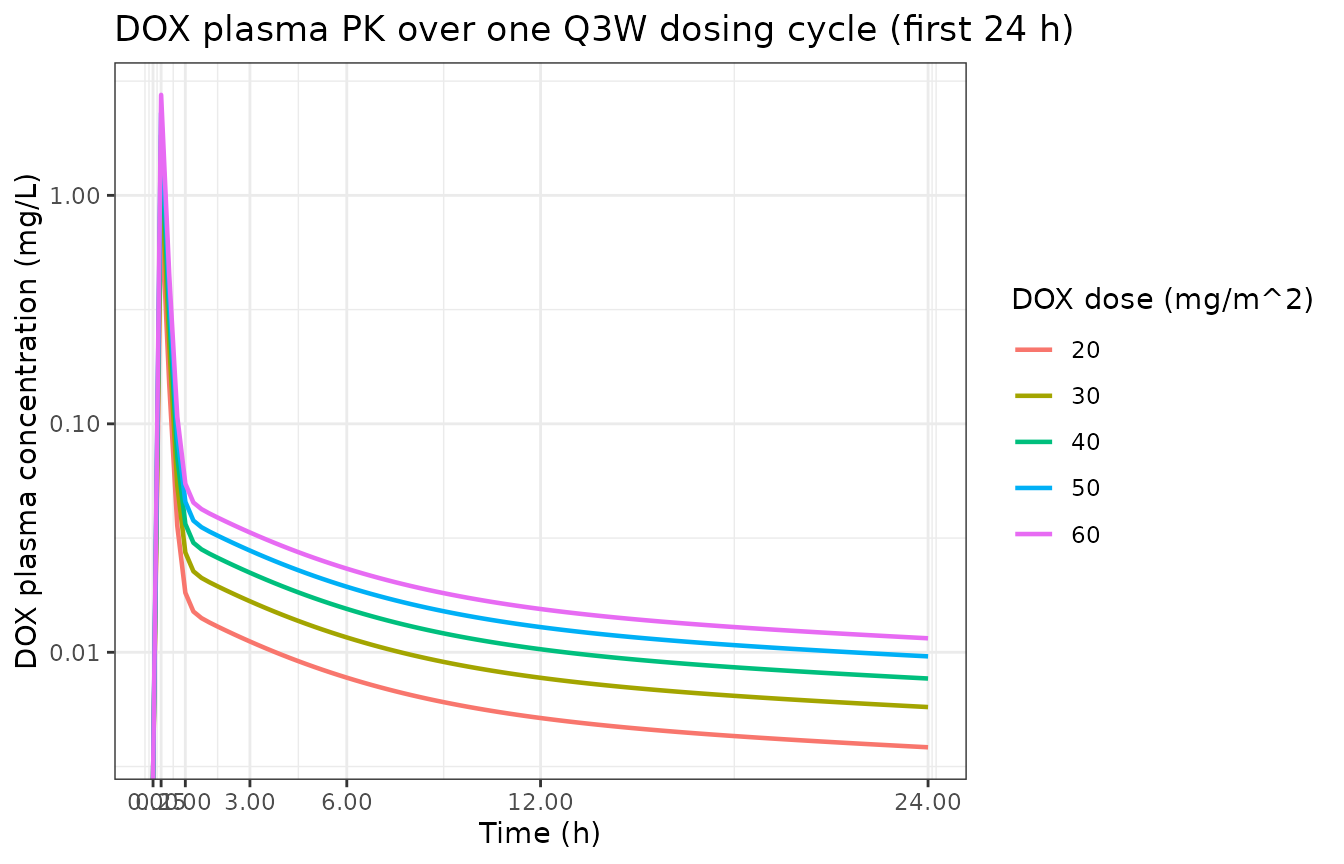
Replicates Mody 2023 Figure 4B: single-cycle DOX plasma concentration over 24 h at 20, 30, 40, 50, 60 mg/m^2.
Figures 4C and 4D - DEX plasma PK at DEX:DOX = 10:1 (representative)
# 500 mg/m^2 DEX -> 900 mg for BSA=1.8
dex_dose_mg <- 500 * bsa
ev_dex <- purrr::reduce(q3w_times, function(acc, t0) {
  rxode2::et(acc, amt = 90,  rate = 90  / 0.25, cmt = "central",     time = t0) |>
    rxode2::et(amt = dex_dose_mg,
               rate = dex_dose_mg / 0.25, cmt = "central_dex", time = t0)
}, .init = rxode2::et()) |>
  rxode2::et(obs_grid, cmt = "Cc_dex")

sim_dex_pk <- as.data.frame(rxode2::rxSolve(mod_typical, ev_dex, useLinCmt = FALSE))

p_left <- ggplot(sim_dex_pk, aes(x = time / 24 / 7, y = Cc_dex)) +
  geom_line(linewidth = 0.8, color = "steelblue") +
  scale_x_continuous("Time (weeks)", breaks = 0:10) +
  scale_y_log10("DEX plasma (mg/L)") +
  theme_bw() +
  labs(title = "3 cycles Q3W")

p_right <- ggplot(dplyr::filter(sim_dex_pk, time <= 24), aes(x = time, y = Cc_dex)) +
  geom_line(linewidth = 0.8, color = "steelblue") +
  scale_x_continuous("Time (h)", breaks = c(0, 0.25, 1, 3, 6, 12, 24)) +
  scale_y_log10("DEX plasma (mg/L)") +
  theme_bw() +
  labs(title = "First 24 h")

# Use patchwork if available; else plot side by side via cowplot; else print both
if (requireNamespace("patchwork", quietly = TRUE)) {
  print(patchwork::wrap_plots(p_left, p_right, ncol = 2))
} else {
  print(p_left)
  print(p_right)
}
#> Warning in transformation$transform(x): NaNs produced
#> Warning in scale_y_log10("DEX plasma (mg/L)"): log-10 transformation introduced
#> infinite values.
#> Warning: Removed 1 row containing missing values or values outside the scale range
#> (`geom_line()`).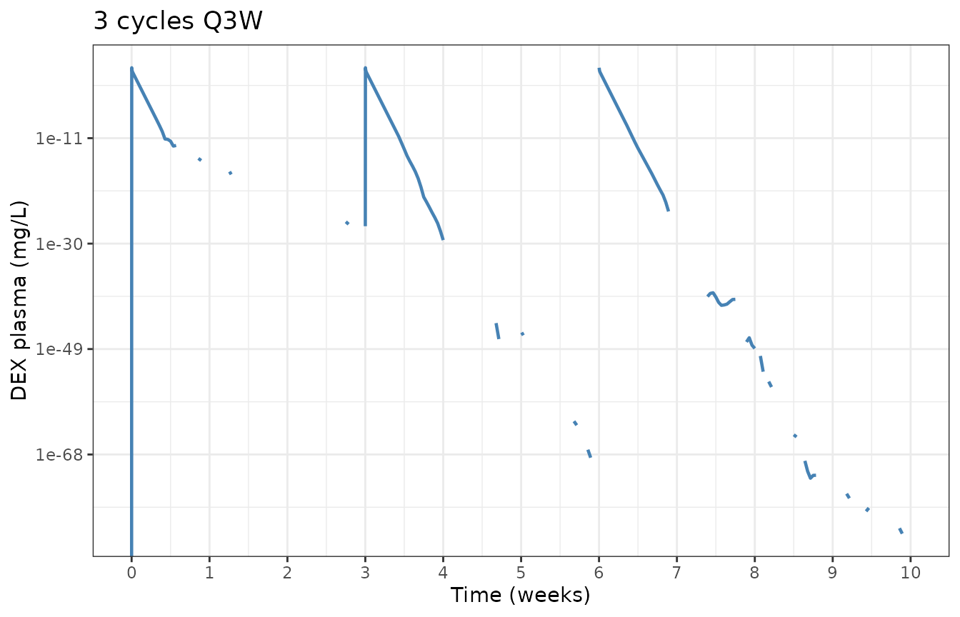
Replicates Mody 2023 Figures 4C-D: representative DEX PK at DEX:DOX = 10:1 (i.e., 500 mg/m^2 DEX with 50 mg/m^2 DOX). Left panel spans three Q3W cycles, right panel zooms to the first 24 h.
#> Warning in scale_y_log10("DEX plasma (mg/L)"): log-10 transformation introduced
#> infinite values.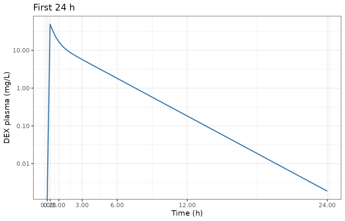
Replicates Mody 2023 Figures 4C-D: representative DEX PK at DEX:DOX = 10:1 (i.e., 500 mg/m^2 DEX with 50 mg/m^2 DOX). Left panel spans three Q3W cycles, right panel zooms to the first 24 h.
Figure 4E – AUEC(DOX+DEX) / AUEC(DOX) at various DEX:DOX dose ratios
Mody 2023 Figure 4E reports the ratio of the area under the effect (cell viability) curve for DOX + DEX to that for DOX alone, evaluated over the three-cycle 9-week window at DEX:DOX dose ratios of 0:1, 1:1, 5:1, 10:1, 20:1, and 50:1 (at 50 mg/m^2 DOX). A ratio > 1 indicates DEX-mediated cardioprotection (higher preserved viability). The paper predicts maximum protection at 10:1 or 20:1.
# Simulate 9-week clinical exposure at fixed 50 mg/m^2 DOX, varying DEX
dox_dose_50 <- mgpm2_to_mg(50)   # 90 mg for BSA 1.8

# Wide observation grid for AUEC
auec_grid <- seq(0, 1512, by = 6)   # 63 days = 9 weeks; 6-h steps
auec_grid <- sort(unique(c(auec_grid, unlist(lapply(q3w_times, obs_dense_by_dose)))))

sim_at_ratio <- function(ratio) {
  dex_amt <- ratio * dox_dose_50
  ev <- purrr::reduce(q3w_times, function(acc, t0) {
    ev1 <- rxode2::et(acc, amt = dox_dose_50, rate = dox_dose_50 / 0.25,
                      cmt = "central", time = t0)
    if (dex_amt > 0) {
      ev1 <- rxode2::et(ev1, amt = dex_amt, rate = dex_amt / 0.25,
                        cmt = "central_dex", time = t0)
    }
    ev1
  }, .init = rxode2::et()) |>
    rxode2::et(auec_grid, cmt = "viability")

  df <- as.data.frame(rxode2::rxSolve(mod_typical, ev, useLinCmt = FALSE)) |>
    dplyr::filter(!is.na(viability))
  # Trapezoidal AUEC of viability (%*h) over the 9-week window
  df <- df |> dplyr::arrange(time)
  auec <- sum(diff(df$time) * (utils::head(df$viability, -1) +
                                utils::tail(df$viability, -1)) / 2)
  data.frame(ratio = ratio, auec = auec)
}

auec_ratios <- c(0, 1, 5, 10, 20, 50)
auec_tbl    <- purrr::map_dfr(auec_ratios, sim_at_ratio)
auec_dox    <- auec_tbl$auec[auec_tbl$ratio == 0]

auec_norm <- auec_tbl |>
  dplyr::mutate(auec_ratio_norm = auec / auec_dox)

ggplot(auec_norm, aes(x = factor(ratio), y = auec_ratio_norm)) +
  geom_col(fill = "steelblue") +
  geom_hline(yintercept = 1, linetype = "dashed", color = "grey30") +
  scale_y_continuous("AUEC(DOX+DEX) / AUEC(DOX)") +
  theme_bw() +
  labs(x = "DEX:DOX dose ratio",
       title = "Cardioprotective effect of DEX at 50 mg/m^2 DOX Q3W (3 cycles)")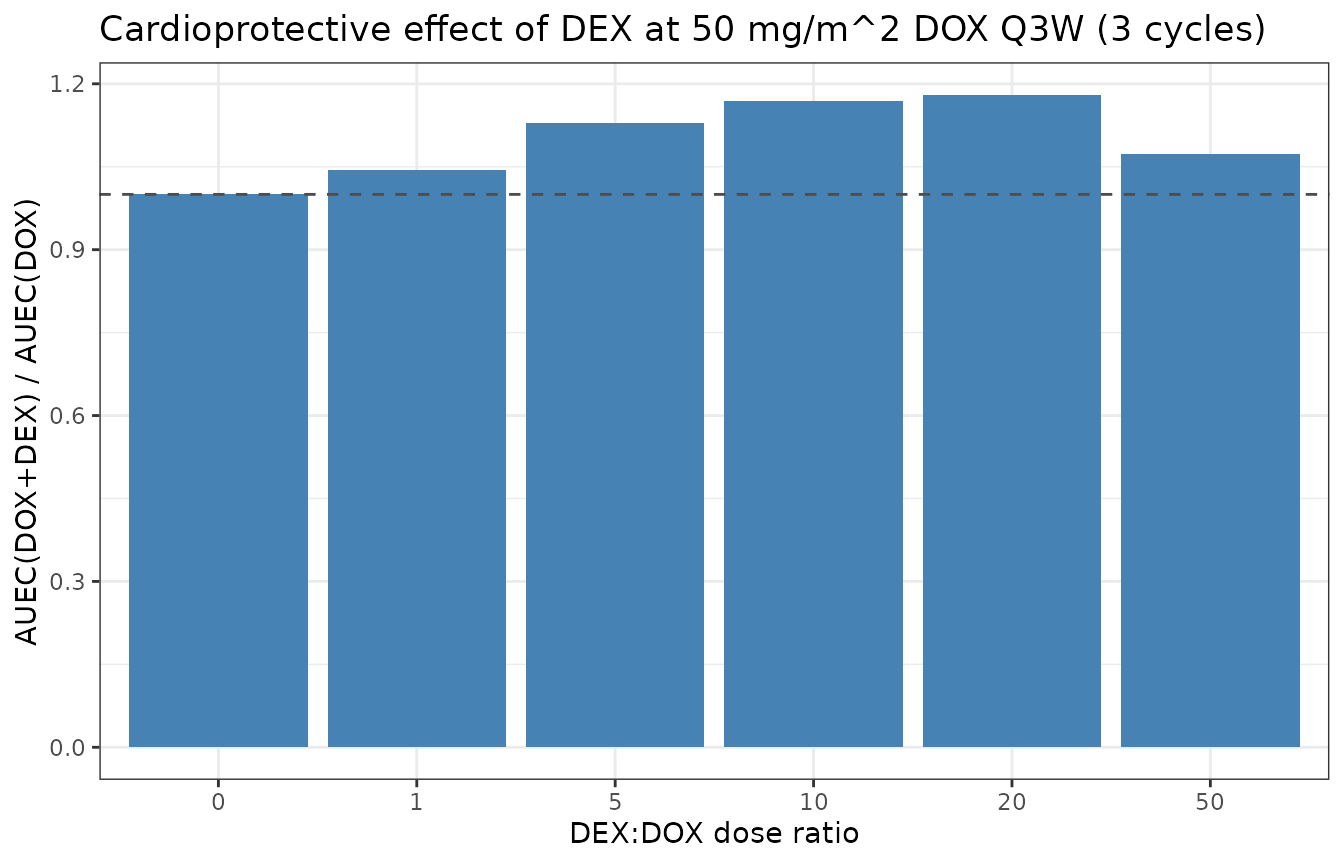
Replicates Mody 2023 Figure 4E: AUEC(DOX+DEX) / AUEC(DOX) ratio at 50 mg/m^2 DOX Q3W for three cycles across DEX:DOX ratios.
Figure 5B/C – Q3W vs. Q1W dose fractionation with DEX
Mody 2023 Figures 5B/C compare the AUEC of viability under (i) 50 mg/m^2 Q3W DOX and (ii) 16.67 mg/m^2 Q1W DOX (dose fractionation), each with or without 10:1 DEX, over three cycles (nine weeks). The paper concludes that Q3W + 10:1 DEX offers the greatest cardioprotection.
# Q3W: 50 mg/m^2 * 1.8 = 90 mg at t = 0, 504, 1008 h
# Q1W: 16.67 mg/m^2 * 1.8 = 30 mg at t = 0, 168, 336, 504, ..., 1176 h
# (nine Q1W doses)
q1w_times <- seq(0, 8 * 168, by = 168)
q1w_dox_mg <- mgpm2_to_mg(16.67)

sim_regimen <- function(regimen, use_dex) {
  if (regimen == "Q3W") {
    dose_times <- q3w_times
    per_dose <- dox_dose_50
  } else {
    dose_times <- q1w_times
    per_dose <- q1w_dox_mg
  }
  # 10:1 DEX with respect to each DOX dose
  ev <- purrr::reduce(dose_times, function(acc, t0) {
    ev1 <- rxode2::et(acc, amt = per_dose, rate = per_dose / 0.25,
                      cmt = "central", time = t0)
    if (use_dex) {
      dex_amt <- 10 * per_dose
      ev1 <- rxode2::et(ev1, amt = dex_amt, rate = dex_amt / 0.25,
                        cmt = "central_dex", time = t0)
    }
    ev1
  }, .init = rxode2::et()) |>
    rxode2::et(auec_grid, cmt = "viability")

  df <- as.data.frame(rxode2::rxSolve(mod_typical, ev, useLinCmt = FALSE)) |>
    dplyr::filter(!is.na(viability)) |>
    dplyr::arrange(time)
  auec <- sum(diff(df$time) * (utils::head(df$viability, -1) +
                                utils::tail(df$viability, -1)) / 2)
  data.frame(regimen = regimen, dex = ifelse(use_dex, "with 10:1 DEX", "no DEX"),
             auec = auec)
}

reg_tbl <- purrr::map_dfr(c("Q3W", "Q1W"), function(r) {
  purrr::map_dfr(c(FALSE, TRUE), function(d) sim_regimen(r, d))
})

reg_norm <- reg_tbl |>
  dplyr::mutate(auec_norm = auec / auec_tbl$auec[auec_tbl$ratio == 0])

ggplot(reg_norm, aes(x = regimen, y = auec_norm, fill = dex)) +
  geom_col(position = position_dodge()) +
  geom_hline(yintercept = 1, linetype = "dashed", color = "grey30") +
  scale_y_continuous("AUEC / AUEC(50 mg/m^2 DOX Q3W, no DEX)") +
  scale_fill_manual(values = c("no DEX" = "grey55", "with 10:1 DEX" = "steelblue")) +
  theme_bw() +
  labs(x = "DOX regimen", fill = "",
       title = "DOX regimen x DEX combination over 9 weeks (3 cycles)")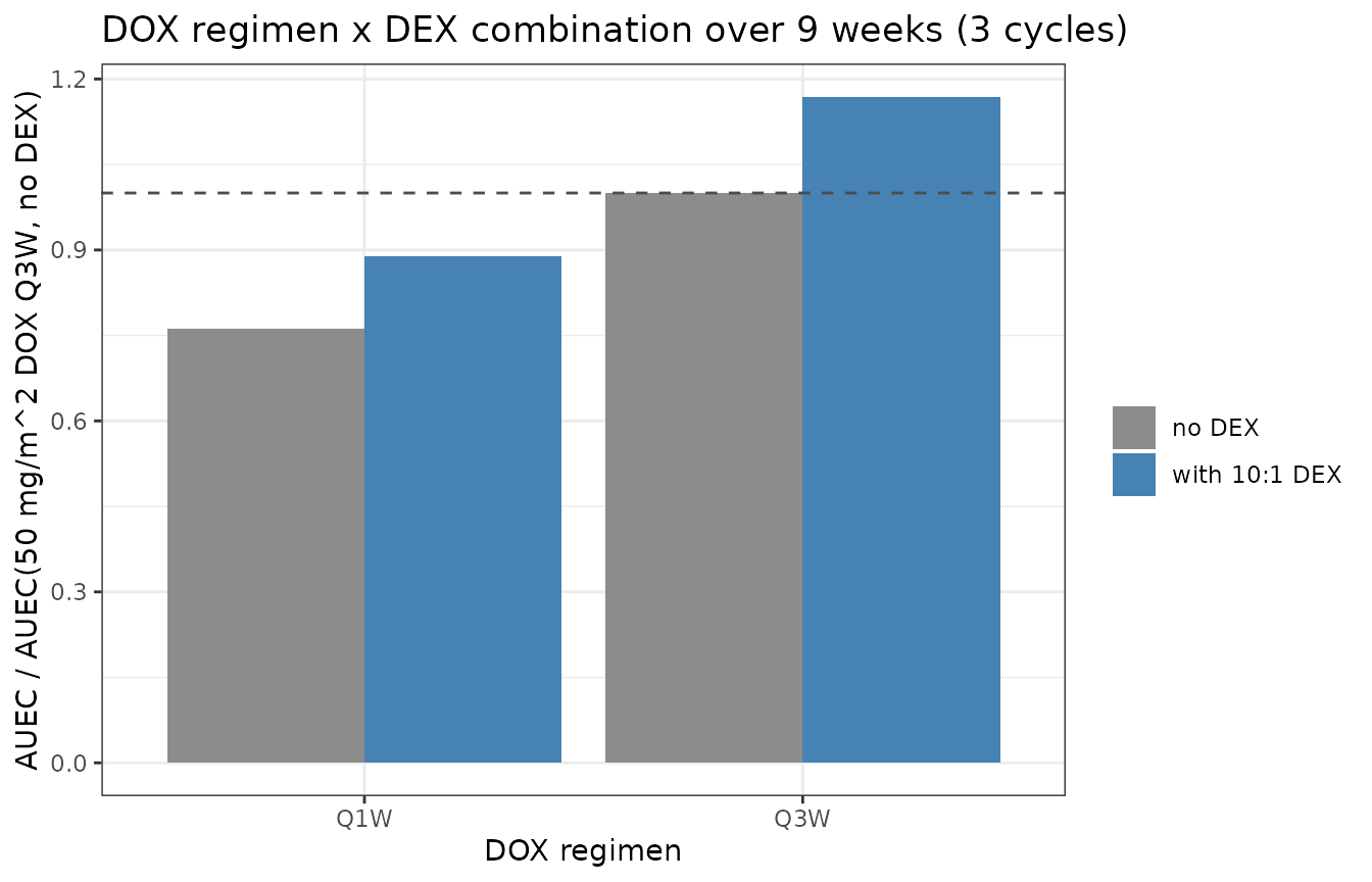
Replicates Mody 2023 Figure 5B/C: AUEC of AC16 cell viability under Q3W vs. Q1W DOX with / without 10:1 DEX, over 9 weeks (3 cycles).
PKNCA validation of clinical DOX PK
Because Mody 2023 does not tabulate NCA parameters (the paper’s Figure 4 shows PK profiles from the clinical model but does not report Cmax / AUC values numerically), the PKNCA block below is a sanity check on the packaged PK: it computes exposure metrics after a single 50 mg/m^2 Q3W IV infusion and reports them as a self-consistency demonstration. The paper’s PK values are drawn from Kontny 2013 (DOX) and Earhart 1982 (DEX); a downstream user wanting to cross-validate the packaged PK should compare against those upstream sources.
# Single-cycle simulation at 50 mg/m^2 DOX + 500 mg/m^2 DEX
one_cycle_grid <- sort(unique(c(seq(0, 24, by = 0.25), seq(24, 504, by = 6))))
ev_single <-
  rxode2::et(amt = dox_dose_50, rate = dox_dose_50 / 0.25,
             cmt = "central", time = 0) |>
  rxode2::et(amt = 900, rate = 900 / 0.25, cmt = "central_dex", time = 0) |>
  rxode2::et(one_cycle_grid, cmt = "Cc") |>
  rxode2::et(one_cycle_grid, cmt = "Cc_dex")
sim_single <- as.data.frame(rxode2::rxSolve(mod_typical, ev_single, useLinCmt = FALSE))

# NCA on DOX plasma. Keep only the Cc-slot rows to avoid duplicated
# (id, time) rows (rxode2 emits one row per output at each observation
# time in a multi-output model).
sim_dox_nca <- sim_single |>
  dplyr::filter(!is.na(Cc), CMT == 10L) |>
  dplyr::transmute(id = 1L, time = time, Cc = Cc, treatment = "DOX 50 mg/m^2 Q3W")

dose_dox <- data.frame(
  id = 1L, time = 0, amt = dox_dose_50, treatment = "DOX 50 mg/m^2 Q3W"
)

conc_obj_dox <- PKNCA::PKNCAconc(sim_dox_nca, Cc ~ time | treatment + id,
                                 concu = "mg/L", timeu = "h")
dose_obj_dox <- PKNCA::PKNCAdose(dose_dox, amt ~ time | treatment + id,
                                 doseu = "mg")

intervals_dox <- data.frame(
  start = 0, end = 504,
  cmax = TRUE, tmax = TRUE, auclast = TRUE, aucinf.obs = TRUE, half.life = TRUE
)
nca_dox <- PKNCA::pk.nca(PKNCA::PKNCAdata(conc_obj_dox, dose_obj_dox,
                                          intervals = intervals_dox))

nca_dox_df <- as.data.frame(nca_dox$result) |>
  dplyr::select(treatment, PPTESTCD, PPORRES) |>
  tidyr::pivot_wider(names_from = PPTESTCD, values_from = PPORRES) |>
  dplyr::rename(
    "Treatment"                = treatment,
    "Cmax (mg/L)"              = cmax,
    "Tmax (h)"                 = tmax,
    "AUClast (0-504 h, mg*h/L)" = auclast,
    "AUCinf,obs (mg*h/L)"      = aucinf.obs,
    "t1/2 (h)"                 = half.life
  )

knitr::kable(nca_dox_df, digits = 3,
caption = "PKNCA-derived DOX exposure metrics for a single 50 mg/m^2 Q3W IV infusion (BSA 1.8 m^2 typical subject).")| Treatment | AUClast (0-504 h, mg*h/L) | Cmax (mg/L) | Tmax (h) | tlast | clast.obs | lambda.z | r.squared | adj.r.squared | lambda.z.time.first | lambda.z.time.last | lambda.z.n.points | clast.pred | t1/2 (h) | span.ratio | AUCinf,obs (mg*h/L) |
|---|---|---|---|---|---|---|---|---|---|---|---|---|---|---|---|
| DOX 50 mg/m^2 Q3W | 1.611 | 2.295 | 0.25 | 504 | 0 | 0.015 | 1 | 1 | 12 | 504 | 129 | 0 | 45.767 | 10.75 | 1.611 |
Assumptions and deviations
The following are paper-vs-model gaps that the maintainers preserved deliberately rather than tuning parameters to close.
DEX inhibition equation form is subtractive on Kmax. The PDF’s formal equations for the combination model (Mody 2023 Eqs 6a-6f) could not be recovered as machine-readable text from the PDF. Table 1 gives Imax,DEXi units of 1/h (matching Kmax,DOX), and the text describes the DEX effect as “a capacity limited Hill function K_DEX … on DOX cell- death stimulation.” The packaged model implements the DEX inhibition as a subtraction on the maximum DOX kill rate constant,
K_source = (Kmax - Imax_DEXi * CDEX / (IC50_DEXi + CDEX)) * CDOX / (KC50 + CDOX), so that at saturating DEX (CDEX >> IC50) the effective maximum kill rate isKmax - Imax_DEXi = 0.0072 /h(about 90% reduction fromKmax = 0.0697 /h). This form is dimensionally consistent, always non-negative for the paper’s parameter values, and matches the qualitative behaviour of Figure 2C (dose-dependent partial cardioprotection). A downstream user with access to the paper’s LaTeX source is encouraged to confirm the functional form and rerun the fit if the printed equation differs.Clinical DOX PK values are reproduced by Mody 2023 from Kontny 2013. Mody 2023 Table 2 top row is a direct restatement of the DOX 3-compartment PK parameters from Kontny NE et al., J Clin Oncol 2013 (paper ref [30]); the Kontny 2013 paper itself was not available when this model was built. The 6 CL / V parameters (CL, Vc, Q2, Vp, Q3, Vp2) match Kontny 2013’s Table 2 to the digits reported in Mody 2023.
Clinical DEX PK values are Mody-2023-fitted to Earhart 1982. DEX PK was originally fit by Mody 2023 to phase 1 human data from Earhart RH et al., Cancer Res 1982 (paper ref [29]) at doses of 50 to 2500 mg/m^2 Q3W. Table 2 bottom reports the micro-constants (kel = 1 /h, k12 = 1 /h, k21 = 1 /h, V = 14.6 L) with RSE 3-8%. The packaged model uses the canonical CL / Vc / Q / Vp macro parameterisation with values back-derived from the micro-constants (CL = kel * V, Q = k12 * V, Vp = V * k12 / k21); all four macro parameters numerically equal 14.6 L or 14.6 L/h.
No IIV in the packaged model. Mody 2023 does not fit IIV; per- parameter %RSEs in Tables 1 and 2 are from the Monolix fit only. The paper Methods section injects an arbitrary 10% CV IIV on TD parameters at simulation time for the 500-subject cohort simulation used to generate Figure 4. A downstream user wanting to replicate that 500-subject spread can add
omegablocks to the model outside the packaged file (or perturb the parameter values manually).Residual error placeholders. Neither Table 1 nor Table 2 reports residual SDs. The packaged model carries small
fixed()placeholder additive residual SDs (addSd = 1 mg/L,addSd_dex = 1 mg/L,addSd_viability = 5%) so that the multi-output model parses cleanly; the values do not represent assay precision.Molecular masses are literature-derived. The mg/L to uM conversion factors (
lconv_dox = log(1.8397)andlconv_dex = log(3.7275)) use PubChem free-base molecular masses (DOX 543.52 g/mol, PubChem CID 31703; DEX 268.27 g/mol, PubChem CID 71384). The paper reports doses as mg/m^2 without specifying salt vs free base; the mg/m^2 -> mg conversion in this vignette treats the doses as free base. Downstream users dosing the HCl salt should scale the amt by 543.52 / 579.98 = 0.937 for DOX to preserve free-base amounts.Figure 5 fractional dose is 16.67 mg/m^2. The paper reports 50 / 3 = 16.67 mg/m^2 Q1W as the dose-fractionated regimen equivalent of 50 mg/m^2 Q3W. Over 9 weeks (3 cycles) the Q3W regimen has 3 doses (150 mg/m^2 total) while Q1W has 9 doses (150.03 mg/m^2 total, essentially matched). Simulation uses the paper’s exact 16.67 mg/m^2 Q1W value; 8 doses at 168-h intervals (t = 0, 168, …, 1176 h) plus the initial dose at t = 0 gives 9 Q1W doses over the 63-day window.
Errata
The model equations (Eqs 1, 2, 3, 4a-e, 5, 6a-f) could not be recovered as machine-readable text from the Mody 2023 PDF. The equation forms used in the packaged model were reconstructed from the surrounding prose, the parameter units in Tables 1 and 2, and the schematic in Figure 1. See the “DEX inhibition equation form” assumption above for the specific interpretation choice.
Mody 2023 Table 1 reports kdeg values in the Results text only (
kdeg_DOX = 0.022 (+/- 0.0004) /h,kdeg_DEX = 0.054 (+/- 0.0016) /h). These are used only in vitro (Supp. Fig. 1 supports them) and are NOT part of the packaged clinical PK / TD model; they are used in the auxiliary in vitro model constructed inline in this vignette to reproduce Figures 2A-C.First author Hardik Mody and second author Tanaya R. Vaidya contributed equally per the paper’s byline footnote. Third author Sihem Ait-Oudhia (Quantitative Pharmacology and Pharmacometrics, Merck & Co.) is the corresponding author. The packaged model filename uses the first-listed author (
Mody_2023_...) per the nlmixr2lib author-surname normalisation rule.