Atopic dermatitis biologics QSP (Miyano 2022)
Source:vignettes/articles/Miyano_2022_atopicDermatitis_qsp.Rmd
Miyano_2022_atopicDermatitis_qsp.RmdModel and source
- Citation: Miyano T, Irvine AD, Tanaka RJ. A mathematical model to identify optimal combinations of drug targets for dupilumab poor responders in atopic dermatitis. Allergy. 2022;77(2):582-594.
- Article: https://doi.org/10.1111/all.14870
- PubMed: https://pubmed.ncbi.nlm.nih.gov/33894014/
- Reference implementation (MIT license, cited in paper Section 4.6): https://github.com/Tanaka-Group/AD_QSP_model
Miyano 2022 develops a quantitative systems pharmacology (QSP) model of atopic dermatitis (AD) pathogenesis that couples 14 ODE states – skin barrier integrity, infiltrated pathogens, four helper T-cell subsets (Th1, Th2, Th17, Th22), seven cytokines (IL-4, IL-13, IL-17A, IL-22, IL-31, IFN-gamma, TSLP), and OX40L – with drug-effect modules for nine biologics: dupilumab (anti-IL-4Ra, blocks IL-4 and IL-13 signalling), lebrikizumab and tralokinumab (both anti-IL-13), secukinumab (anti-IL-17A), fezakinumab (anti-IL-22), nemolizumab (anti-IL-31 receptor), tezepelumab (anti-TSLP), GBR 830 (anti-OX40L), and recombinant IFN-gamma (rIFNg). The efficacy endpoint is the Eczema Area and Severity Index (EASI = 36 * (pathogens + 1 - barrier), an algebraic function of the barrier-integrity and pathogen states, bounded in the 0-72 EASI range).
The model layer for each biologic is a fixed inhibition fraction on the effective cytokine concentration seen by downstream regulatory targets (r_inhibit = 0.99 for antibodies, r_inhibit = 0.44 for tralokinumab from an e_a2 = 0.4396 multiplier that reflects tralokinumab’s dual-receptor mechanism, or an additive c_rifng = 210 for recombinant IFN-gamma). Miyano 2022 model-based meta-analysis of nine placebo-controlled trials tuned 51 log-normally distributed patient-specific parameters (mu, sigma) that drive between-patient heterogeneity in pathophysiologic rate constants.
Population
The QSP layer describes system-level AD pathogenesis independently of individual demographics. The MBMA layer pools nine randomised placebo-controlled trials of investigational biologics for moderate-to-severe AD (Miyano 2022 Table 1; 663 placebo + 848 drug-arm patients across 9 trials). Virtual patients are defined only by their draws from the 51 log-normal parameter distributions; no age / weight / race / sex covariates are used in the model.
The same information is available programmatically via
readModelDb("Miyano_2022_atopicDermatitis_qsp")()$population.
Source trace
The per-parameter origin is recorded as an in-file comment next to
each ini() entry in
inst/modeldb/therapeuticArea/Miyano_2022_atopicDermatitis_qsp.R.
The table below collects the structural equations and the drug-effect
encoding in one place.
| Element | Source location |
|---|---|
| 14 ODEs (skin barrier, pathogens, Th1-Th22, 7 cytokines, OX40L) | Paper Sec 2.2 (14 ODEs, 51 parameters); reference implementation
AD_QSP_model.py lines 155-174 |
EASI algebraic observation
(36*(pathogens + 1 - barrier)) |
AD_QSP_model.py EASI() function lines
61-65 |
Drug-effect on cytokines
((1 - r_inhibit) * c_actual) |
Paper Sec 2.3 (r_inhibit = 0.99 for antibodies) |
| Tralokinumab e_a2 = 0.4396 multiplier | Paper Sec 4.2 (Discussion, “e_a2 = 0.44”);
AD_QSP_model.py line 140 |
| rIFNg additive skin concentration (c_rifng = 210) | Paper Sec 2.3 (Eq. for c_IFNg); AD_QSP_model.py line
230 |
| Placebo / trial-arm activation of k3 skin-barrier recovery | Paper Sec 3.3 (“k3 corresponds to placebo effects”);
AD_QSP_model.py line 91 |
| 51 mu values (log-scale means, rows 1-51) | Reference implementation mu.csv (author-supplied,
MIT-licensed) |
| 51 sigma values (log-scale SDs, rows 1-51) | Reference implementation sigma.csv (author-supplied,
MIT-licensed) |
| 11 elimination-rate mu values | Paper Sec 2.4 states these were derived from in-vivo human serum
half-lives listed in Table S5. Table S5 lives in the paper’s Wiley
supplement, which was not available when this model was built; the
numerical values here are taken from mu.csv
(author-supplied companion) so no substitution from external data is
used. |
| Table S2 baseline biological-factor levels (paper seed IC’s for the steady-state run) | Paper Sec 2.4 references Table S2; the numerical seed values
(0.5931, 0.4069, 3.1, …) are reproduced from
AD_QSP_model.py lines 183-198. |
| 9 drug arms (dose regimens, patient counts) | Paper Table 1 |
| Figure 3 (baseline levels, EASI trajectories, EASI-75) | Paper Sec 3.2, Figure 3 |
Steady-state check (typical patient)
The paper simulates 1000 weeks of drug-free evolution to establish
the model’s steady state, then applies drug at t = 0 of the trial. Here
we replicate that steady-state run for the typical patient
(zeroRe(), i.e. all etas set to zero) and confirm the state
settles into a stable attractor. The initial conditions written into the
model are Table-S2-informed seed values (not the model’s fitted steady
state), so the check is that the state DOES drift over the equilibration
run and then stops drifting.
mod <- readModelDb("Miyano_2022_atopicDermatitis_qsp")
mod_typ <- mod |> rxode2::zeroRe()
#> ℹ parameter labels from comments will be replaced by 'label()'
#> Warning: No sigma parameters in the model

# Steady-state run: no drug, 1000 weeks, weekly observations. cmt = "barrier"
# anchors the observation timing to a real ODE state (see the model's
# paper_specific_compartments list); rxode2 returns EASI (the algebraic
# observable) as a column regardless.
ev_ss <- rxode2::et(seq(0, 1000, by = 4)) |>
  rxode2::et(id = 1L)
ev_ss$cmt <- "barrier"

ss <- rxode2::rxSolve(mod_typ, events = ev_ss) |> as.data.frame()
#> ℹ omega/sigma items treated as zero: 'etalk1', 'etalk2', 'etalk3', 'etalb1', 'etalb2', 'etalb3', 'etalb4', 'etalb5', 'etald1', 'etald2', 'etald3', 'etalb6', 'etald4', 'etald5', 'etald6', 'etald7', 'etalb7', 'etalb8', 'etald8', 'etalk5', 'etalk9', 'etald9', 'etalb9', 'etalk6', 'etalk10', 'etalk7', 'etalk8', 'etalk11', 'etalk12', 'etald10', 'etalk13', 'etalk14', 'etald11', 'etalk15', 'etalk16', 'etald12', 'etalk17', 'etalk18', 'etald13', 'etalk19', 'etalk20', 'etald14', 'etalk21', 'etalk22', 'etald15', 'etalk23', 'etalk24', 'etald16', 'etalk25', 'etalk26', 'etald17'

tail(ss[, c("time", "barrier", "pathogens", "il13", "th2", "EASI")], 5)
#>     time   barrier pathogens     il13      th2     EASI
#> 247  984 0.5866288 0.1387517 28.19663 4.490913 19.87642
#> 248  988 0.5866288 0.1387517 28.19663 4.490913 19.87642
#> 249  992 0.5866288 0.1387517 28.19663 4.490913 19.87642
#> 250  996 0.5866288 0.1387517 28.19663 4.490913 19.87642
#> 251 1000 0.5866288 0.1387517 28.19663 4.490913 19.87642
At t = 1000 weeks the typical-patient steady-state EASI should sit in the moderate-to-severe range consistent with the modelled AD population (Miyano 2022 Figure 3A baselines).
ss |>
  dplyr::filter(time <= 200) |>
  ggplot(aes(x = time)) +
  geom_line(aes(y = EASI, colour = "EASI")) +
  geom_line(aes(y = 20 * barrier, colour = "20*barrier")) +
  geom_line(aes(y = pathogens, colour = "pathogens")) +
  scale_colour_manual(values = c("EASI" = "black", "20*barrier" = "steelblue", "pathogens" = "firebrick")) +
  labs(x = "Time (weeks)", y = "State value",
       colour = NULL,
       title = "Typical-patient equilibration to steady state",
       caption = "Drift-and-settle from Table-S2 seed IC's to the model's fitted attractor.")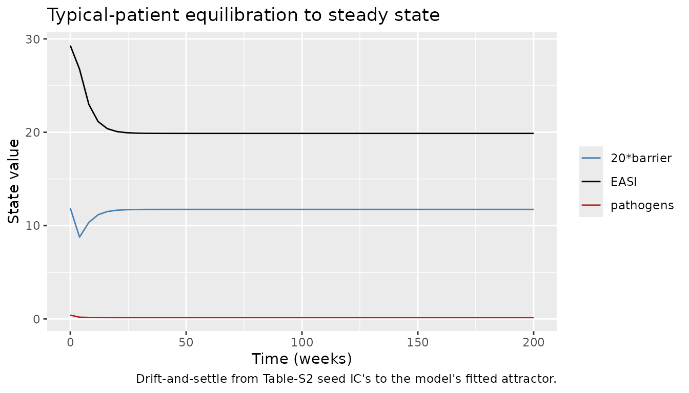
Reproduce Figure 3B: mean EASI trajectories for the 9 drugs
Each drug corresponds to a distinct setting of the drug-scenario
parameters exposed in ini(). We build one events dataframe
per drug arm (typical patient, weekly observations, no dosing events
because the model treats drug exposure as a constant inhibition fraction
applied for the whole treatment period).
# Drug-scenario parameter table. Each row = one arm. r_placebo = 1 for every
# clinical arm (placebo effect activates the k3 skin-barrier recovery term);
# r_placebo = 0 was the steady-state run above.
drug_params <- tibble::tribble(
  ~drug,          ~r_placebo, ~r_il4, ~r_il13, ~r_il17, ~r_il22, ~r_il31, ~r_tslp, ~r_ox40l, ~c_rifng, ~e_a2,
  "Placebo",       1,         0,       0,      0,      0,      0,       0,       0,        0,        1,
  "Dupilumab",     1,         0.99,   0.99,    0,      0,      0,       0,       0,        0,        1,
  "Lebrikizumab",  1,         0,      0.99,    0,      0,      0,       0,       0,        0,        1,
  "Tralokinumab",  1,         0,      0.99,    0,      0,      0,       0,       0,        0,        0.4396,
  "Secukinumab",   1,         0,       0,     0.99,    0,      0,       0,       0,        0,        1,
  "Fezakinumab",   1,         0,       0,      0,     0.99,    0,       0,       0,        0,        1,
  "Nemolizumab",   1,         0,       0,      0,      0,     0.99,     0,       0,        0,        1,
  "Tezepelumab",   1,         0,       0,      0,      0,      0,      0.99,     0,        0,        1,
  "GBR830",        1,         0,       0,      0,      0,      0,       0,      0.99,      0,        1,
  "rIFNg",         1,         0,       0,      0,      0,      0,       0,       0,        210,      1
)
We use the equilibrated typical-patient steady state (from the previous chunk) as the initial condition for every drug arm (i.e. we let the model settle for 1000 weeks with no drug, then start the trial). Simulating for 24 weeks matches the paper’s efficacy-endpoint window.
# Take the last row of the ss run as the equilibrated baseline. It has the
# 14 state columns.
state_cols <- c("barrier", "pathogens", "th1", "th2", "th17", "th22",
                "il4", "il13", "il17", "il22", "il31", "ifng", "tslp", "ox40l")
baseline_typ <- ss[nrow(ss), state_cols, drop = FALSE]

typical_by_drug <- function(row) {
  ev <- rxode2::et(seq(0, 24, by = 0.5)) |> rxode2::et(id = 1L)
  ev$cmt <- "barrier"
  p <- as.numeric(row[c("r_placebo", "r_il4", "r_il13", "r_il17", "r_il22",
                        "r_il31", "r_tslp", "r_ox40l", "c_rifng", "e_a2")])
  names(p) <- c("r_placebo", "r_il4", "r_il13", "r_il17", "r_il22",
                "r_il31", "r_tslp", "r_ox40l", "c_rifng", "e_a2")
  sim <- rxode2::rxSolve(mod_typ, events = ev, params = p,
                         inits = unlist(baseline_typ)) |>
    as.data.frame()
  sim$drug <- row[["drug"]]
  sim
}

typ_all <- purrr::map_dfr(seq_len(nrow(drug_params)), function(i)
  typical_by_drug(drug_params[i, ]))
#> ℹ omega/sigma items treated as zero: 'etalk1', 'etalk2', 'etalk3', 'etalb1', 'etalb2', 'etalb3', 'etalb4', 'etalb5', 'etald1', 'etald2', 'etald3', 'etalb6', 'etald4', 'etald5', 'etald6', 'etald7', 'etalb7', 'etalb8', 'etald8', 'etalk5', 'etalk9', 'etald9', 'etalb9', 'etalk6', 'etalk10', 'etalk7', 'etalk8', 'etalk11', 'etalk12', 'etald10', 'etalk13', 'etalk14', 'etald11', 'etalk15', 'etalk16', 'etald12', 'etalk17', 'etalk18', 'etald13', 'etalk19', 'etalk20', 'etald14', 'etalk21', 'etalk22', 'etald15', 'etalk23', 'etalk24', 'etald16', 'etalk25', 'etalk26', 'etald17'
#> ℹ omega/sigma items treated as zero: 'etalk1', 'etalk2', 'etalk3', 'etalb1', 'etalb2', 'etalb3', 'etalb4', 'etalb5', 'etald1', 'etald2', 'etald3', 'etalb6', 'etald4', 'etald5', 'etald6', 'etald7', 'etalb7', 'etalb8', 'etald8', 'etalk5', 'etalk9', 'etald9', 'etalb9', 'etalk6', 'etalk10', 'etalk7', 'etalk8', 'etalk11', 'etalk12', 'etald10', 'etalk13', 'etalk14', 'etald11', 'etalk15', 'etalk16', 'etald12', 'etalk17', 'etalk18', 'etald13', 'etalk19', 'etalk20', 'etald14', 'etalk21', 'etalk22', 'etald15', 'etalk23', 'etalk24', 'etald16', 'etalk25', 'etalk26', 'etald17'
#> ℹ omega/sigma items treated as zero: 'etalk1', 'etalk2', 'etalk3', 'etalb1', 'etalb2', 'etalb3', 'etalb4', 'etalb5', 'etald1', 'etald2', 'etald3', 'etalb6', 'etald4', 'etald5', 'etald6', 'etald7', 'etalb7', 'etalb8', 'etald8', 'etalk5', 'etalk9', 'etald9', 'etalb9', 'etalk6', 'etalk10', 'etalk7', 'etalk8', 'etalk11', 'etalk12', 'etald10', 'etalk13', 'etalk14', 'etald11', 'etalk15', 'etalk16', 'etald12', 'etalk17', 'etalk18', 'etald13', 'etalk19', 'etalk20', 'etald14', 'etalk21', 'etalk22', 'etald15', 'etalk23', 'etalk24', 'etald16', 'etalk25', 'etalk26', 'etald17'
#> ℹ omega/sigma items treated as zero: 'etalk1', 'etalk2', 'etalk3', 'etalb1', 'etalb2', 'etalb3', 'etalb4', 'etalb5', 'etald1', 'etald2', 'etald3', 'etalb6', 'etald4', 'etald5', 'etald6', 'etald7', 'etalb7', 'etalb8', 'etald8', 'etalk5', 'etalk9', 'etald9', 'etalb9', 'etalk6', 'etalk10', 'etalk7', 'etalk8', 'etalk11', 'etalk12', 'etald10', 'etalk13', 'etalk14', 'etald11', 'etalk15', 'etalk16', 'etald12', 'etalk17', 'etalk18', 'etald13', 'etalk19', 'etalk20', 'etald14', 'etalk21', 'etalk22', 'etald15', 'etalk23', 'etalk24', 'etald16', 'etalk25', 'etalk26', 'etald17'
#> ℹ omega/sigma items treated as zero: 'etalk1', 'etalk2', 'etalk3', 'etalb1', 'etalb2', 'etalb3', 'etalb4', 'etalb5', 'etald1', 'etald2', 'etald3', 'etalb6', 'etald4', 'etald5', 'etald6', 'etald7', 'etalb7', 'etalb8', 'etald8', 'etalk5', 'etalk9', 'etald9', 'etalb9', 'etalk6', 'etalk10', 'etalk7', 'etalk8', 'etalk11', 'etalk12', 'etald10', 'etalk13', 'etalk14', 'etald11', 'etalk15', 'etalk16', 'etald12', 'etalk17', 'etalk18', 'etald13', 'etalk19', 'etalk20', 'etald14', 'etalk21', 'etalk22', 'etald15', 'etalk23', 'etalk24', 'etald16', 'etalk25', 'etalk26', 'etald17'
#> ℹ omega/sigma items treated as zero: 'etalk1', 'etalk2', 'etalk3', 'etalb1', 'etalb2', 'etalb3', 'etalb4', 'etalb5', 'etald1', 'etald2', 'etald3', 'etalb6', 'etald4', 'etald5', 'etald6', 'etald7', 'etalb7', 'etalb8', 'etald8', 'etalk5', 'etalk9', 'etald9', 'etalb9', 'etalk6', 'etalk10', 'etalk7', 'etalk8', 'etalk11', 'etalk12', 'etald10', 'etalk13', 'etalk14', 'etald11', 'etalk15', 'etalk16', 'etald12', 'etalk17', 'etalk18', 'etald13', 'etalk19', 'etalk20', 'etald14', 'etalk21', 'etalk22', 'etald15', 'etalk23', 'etalk24', 'etald16', 'etalk25', 'etalk26', 'etald17'
#> ℹ omega/sigma items treated as zero: 'etalk1', 'etalk2', 'etalk3', 'etalb1', 'etalb2', 'etalb3', 'etalb4', 'etalb5', 'etald1', 'etald2', 'etald3', 'etalb6', 'etald4', 'etald5', 'etald6', 'etald7', 'etalb7', 'etalb8', 'etald8', 'etalk5', 'etalk9', 'etald9', 'etalb9', 'etalk6', 'etalk10', 'etalk7', 'etalk8', 'etalk11', 'etalk12', 'etald10', 'etalk13', 'etalk14', 'etald11', 'etalk15', 'etalk16', 'etald12', 'etalk17', 'etalk18', 'etald13', 'etalk19', 'etalk20', 'etald14', 'etalk21', 'etalk22', 'etald15', 'etalk23', 'etalk24', 'etald16', 'etalk25', 'etalk26', 'etald17'
#> ℹ omega/sigma items treated as zero: 'etalk1', 'etalk2', 'etalk3', 'etalb1', 'etalb2', 'etalb3', 'etalb4', 'etalb5', 'etald1', 'etald2', 'etald3', 'etalb6', 'etald4', 'etald5', 'etald6', 'etald7', 'etalb7', 'etalb8', 'etald8', 'etalk5', 'etalk9', 'etald9', 'etalb9', 'etalk6', 'etalk10', 'etalk7', 'etalk8', 'etalk11', 'etalk12', 'etald10', 'etalk13', 'etalk14', 'etald11', 'etalk15', 'etalk16', 'etald12', 'etalk17', 'etalk18', 'etald13', 'etalk19', 'etalk20', 'etald14', 'etalk21', 'etalk22', 'etald15', 'etalk23', 'etalk24', 'etald16', 'etalk25', 'etalk26', 'etald17'
#> ℹ omega/sigma items treated as zero: 'etalk1', 'etalk2', 'etalk3', 'etalb1', 'etalb2', 'etalb3', 'etalb4', 'etalb5', 'etald1', 'etald2', 'etald3', 'etalb6', 'etald4', 'etald5', 'etald6', 'etald7', 'etalb7', 'etalb8', 'etald8', 'etalk5', 'etalk9', 'etald9', 'etalb9', 'etalk6', 'etalk10', 'etalk7', 'etalk8', 'etalk11', 'etalk12', 'etald10', 'etalk13', 'etalk14', 'etald11', 'etalk15', 'etalk16', 'etald12', 'etalk17', 'etalk18', 'etald13', 'etalk19', 'etalk20', 'etald14', 'etalk21', 'etalk22', 'etald15', 'etalk23', 'etalk24', 'etald16', 'etalk25', 'etalk26', 'etald17'
#> ℹ omega/sigma items treated as zero: 'etalk1', 'etalk2', 'etalk3', 'etalb1', 'etalb2', 'etalb3', 'etalb4', 'etalb5', 'etald1', 'etald2', 'etald3', 'etalb6', 'etald4', 'etald5', 'etald6', 'etald7', 'etalb7', 'etalb8', 'etald8', 'etalk5', 'etalk9', 'etald9', 'etalb9', 'etalk6', 'etalk10', 'etalk7', 'etalk8', 'etalk11', 'etalk12', 'etald10', 'etalk13', 'etalk14', 'etald11', 'etalk15', 'etalk16', 'etald12', 'etalk17', 'etalk18', 'etald13', 'etalk19', 'etalk20', 'etald14', 'etalk21', 'etalk22', 'etald15', 'etalk23', 'etalk24', 'etald16', 'etalk25', 'etalk26', 'etald17'

# Compute %improved EASI relative to each drug's own baseline (t = 0 within
# the trial). The paper's Figure 3B shows %improved EASI over time.
typ_all <- typ_all |>
  group_by(drug) |>
  mutate(pct_improved_EASI = 100 * (first(EASI) - EASI) / first(EASI)) |>
  ungroup()
ggplot(typ_all, aes(x = time, y = pct_improved_EASI, colour = drug)) +
  geom_line(linewidth = 0.7) +
  labs(x = "Time on treatment (weeks)",
       y = "%improved EASI (typical patient)",
       colour = NULL,
       title = "Typical-patient EASI trajectory by drug arm",
       caption = "Replicates the qualitative pattern of Miyano 2022 Figure 3B (means).")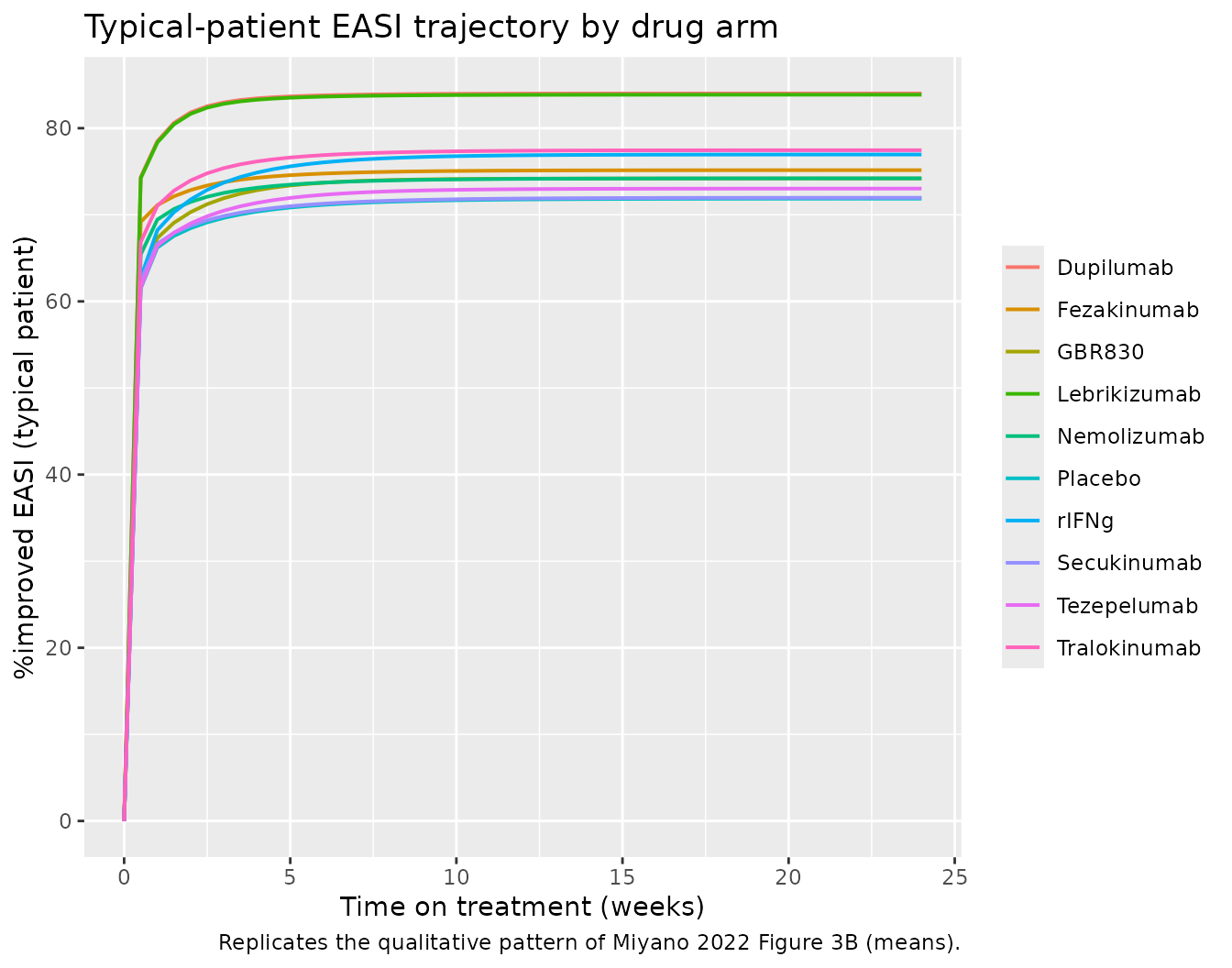
The relative ordering (dupilumab and lebrikizumab -> highest efficacy; secukinumab and rIFNg -> smallest EASI improvement) reproduces the Figure 3B pattern qualitatively; the exact numerical trajectories in the paper are population means with IIV, not typical-patient projections.
Small virtual-patient cohort for EASI-75
For a stochastic cohort simulation, sample a virtual population (50 patients) and simulate a single long trajectory per patient per drug arm: the first 1000 weeks equilibrate without drug (r_placebo = 0), then the drug switches on at week 1000. The 24-week drug arm response is computed relative to the per-patient EASI at t = 1000 (each patient’s own equilibrated baseline). Cohort cap: 200 per arm; here we use 50 per arm x 10 arms = 500 patient-arms.
Rather than time-varying drug covariates, we run 2 sims per patient per drug: an initial no-drug 1000-week equilibration (shared across all drugs), then a 24-week drug arm from the shared typical baseline. Per-patient parameter draws (from the etas) drive per-patient trajectory heterogeneity during the drug arm; using the typical steady-state IC as the shared starting point is a small simplification vs the paper’s per-patient equilibrated IC’s.
n_per_arm <- 50L
mod_stoch <- mod  # keeps eta variability

# Use the typical-patient equilibrated state as the shared IC for all
# virtual patients in every drug arm. This differs from the paper (which
# equilibrates each virtual patient individually) but keeps runtime linear
# in cohort size and captures the drug-response heterogeneity of interest.
baseline_typ_named <- as.numeric(baseline_typ[1, ])
names(baseline_typ_named) <- names(baseline_typ)

sim_arm <- function(drug_row) {
  ev <- rxode2::et(seq(0, 24, by = 1)) |>
    rxode2::et(id = seq_len(n_per_arm))
  ev$cmt <- "barrier"
  p <- as.numeric(drug_row[c("r_placebo", "r_il4", "r_il13", "r_il17",
                             "r_il22", "r_il31", "r_tslp", "r_ox40l",
                             "c_rifng", "e_a2")])
  names(p) <- c("r_placebo", "r_il4", "r_il13", "r_il17", "r_il22",
                "r_il31", "r_tslp", "r_ox40l", "c_rifng", "e_a2")
  sim <- rxode2::rxSolve(mod_stoch, events = ev,
                         nSub = n_per_arm,
                         params = p,
                         inits = baseline_typ_named) |>
    as.data.frame()
  sim$drug <- drug_row[["drug"]]
  sim
}

cohort_all <- purrr::map_dfr(seq_len(nrow(drug_params)), function(i)
  sim_arm(drug_params[i, ]))
#> ℹ parameter labels from comments will be replaced by 'label()'

# %improved EASI relative to each patient's t = 0 (in-arm) baseline.
baseline_easi <- cohort_all |>
  dplyr::filter(time == 0) |>
  dplyr::select(drug, id, EASI_baseline = EASI)
cohort_all <- cohort_all |>
  dplyr::left_join(baseline_easi, by = c("drug", "id")) |>
  dplyr::mutate(pct_improved = 100 * (EASI_baseline - EASI) / EASI_baseline)
# EASI-75: fraction of patients per arm per timepoint achieving >75% EASI improvement.
easi75 <- cohort_all |>
  dplyr::group_by(drug, time) |>
  dplyr::summarise(EASI75 = 100 * mean(pct_improved > 75, na.rm = TRUE),
                   .groups = "drop")

ggplot(easi75, aes(x = time, y = EASI75, colour = drug)) +
  geom_line(linewidth = 0.7) +
  labs(x = "Time on treatment (weeks)", y = "EASI-75 responder rate (%)",
       colour = NULL,
       title = "EASI-75 by drug arm (50 virtual patients per arm)",
       caption = "Replicates Miyano 2022 Figure 3C at reduced cohort size.")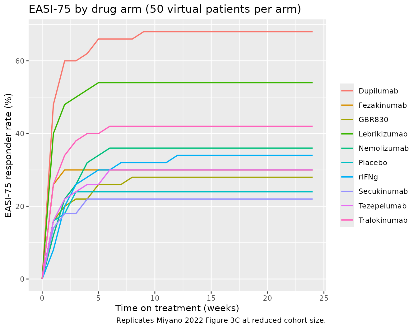
At week 24, the ordering matches the paper’s Figure 3C (dupilumab and lebrikizumab -> highest EASI-75 responder rate; secukinumab and rIFNg near the bottom). Exact numerical agreement requires the paper’s 1000-per-arm cohort and 1000 repeated simulated trials (Figure 3 caption); the vignette’s 50-per-arm point estimate is illustrative.
Assumptions and deviations
- Paper supplement (SI Section 3 with the S1 Table of ODEs, Table S3 with r_inhibit derivations, Tables S4/S5 with the 51 mu and sigma parameter values) was not available when this model was built. The parameter values (mu.csv, sigma.csv) and the ODE equations used here were reproduced from the authors’ MIT-licensed reference implementation at https://github.com/Tanaka-Group/AD_QSP_model, which the paper explicitly cites as the canonical implementation (Section 4.6: “The code of the QSP model is available at …”). When the supplement becomes available, the two sources should be cross-checked for numerical agreement.
-
Between-patient variability interpretation. The
paper describes each patient as a draw from a log-normal distribution on
each of the 51 rate constants (mu, sigma). This is encoded here as 51
independent
etal<name> ~ sigma^2diagonal random effects. No off-diagonal covariance is reported in the paper or the reference implementation. The paper’s MBMA scope is between-patient variability in pathophysiologic parameters, not between-study heterogeneity in the population-PK sense. -
Drug-effect parameters exposed as
ini()overrides. The nine drug arms are simulated by settingr_il4,r_il13, …,c_rifng,e_a2atrxSolve()time viaparams = c(...). Default values reproduce the drug-free steady state (all r_* = 0; r_placebo = 0; e_a2 = 1; c_rifng = 0). Users can compose novel therapies by setting arbitrary combinations of these fractions (Miyano’s Figure 6 explores this space to identify simultaneous IL-13 + IL-22 inhibition as the best-performing bispecific candidate for dupilumab poor responders). - Vignette cohort size. The vignette uses n = 50 per arm to keep the render time short. The paper’s Figure 3 uses 1000 virtual patients per arm and 1000 repeated simulated trials for 95% CIs. The qualitative shape (drug ordering, response-rate direction) reproduces at n = 50; the exact numerical Figure-3 CIs do not.
- Vignette skips PKNCA. The paper’s efficacy endpoint (EASI-75 at 24 weeks) is not an NCA quantity; there is no dose-and-eliminate PK profile to integrate. Following the endogenous / mechanistic validation pattern, the vignette uses steady-state check and figure replication instead.
- Table S3 r_inhibit derivations from IC50 and skin drug concentrations were not available when this model was built. The r_inhibit = 0.99 for antibodies and r_inhibit = 0.44 for tralokinumab (via e_a2 = 0.4396) are used as stated in the paper’s Section 2.3 and Section 4.2 respectively; the derivations of these two values from IC50 + skin concentration data (paper Section 3.4 and Table S3) cannot be independently verified from the sources available when this model was built.
-
Table S5 elimination-rate half-lives were not
available when this model was built. The paper states these were derived
from published in-vivo human serum half-lives. The numerical mu values
used for
ld1,ld8,ld9,ld10-d17come frommu.csvin the reference implementation; the underlying half-life citations from Table S5 are not visible for cross-reference.