CD19 CAR T-cell CK/PD QSP (Minucci 2024)
Source:vignettes/articles/Minucci_2024_CART_qsp.Rmd
Minucci_2024_CART_qsp.RmdModel and source
- Citation: Minucci S, Gruver S, Subramanian K, Renardy M (2024). A multi-scale semi-mechanistic CK/PD model for CAR T-cell therapy. Frontiers in Systems Biology 4:1380018. doi:10.3389/fsysb.2024.1380018. Calibrated to CAR T CK / B-cell aplasia data from Ying et al. 2021 (BMC Cancer 21:198; doi:10.1186/s12885-021-07934-1) for the IM19 CD19-targeted CAR T-cell product in 13 relapsed/refractory B-cell non-Hodgkin lymphoma patients.
- Description: QSP (cellular kinetic / pharmacodynamic). Multi-scale semi-mechanistic model for CD19-targeted CAR T-cell therapy of B-cell non-Hodgkin lymphoma. Six T-cell state compartments (infused, effector, memory) for CD8+ and CD4+ phenotypes plus tumor / B cells and endogenous lymphocytes. Effective activation and killing rates are proportional to the CAR fraction bound to CD19, computed as a Hill-type function of tumor burden under the paper’s constant-receptor-density assumption. Per-patient parameters (body weight, CD8 fraction of drug product, initial tumor burden, number of activated-T-cell divisions, memory-cell fraction) come from the fits to n=13 relapsed/refractory NHL patients in Ying et al. 2021. Calibrated to CAR T CK, B-cell aplasia, and structural drug-product characteristics.
- Article: Front. Syst. Biol. 4:1380018
Minucci et al. present a multi-scale semi-mechanistic cellular-kinetic / pharmacodynamic (CK/PD) QSP model for CD19-targeted CAR T-cell therapy of B-cell non-Hodgkin lymphoma. The model was implemented in Applied BioMath’s proprietary QSP platform and calibrated to phase I IM19 CAR T-cell CK and B-cell aplasia data from Ying et al. 2021 (n = 13 relapsed/refractory NHL patients).
Population
Ying et al. 2021 enrolled 13 adults (>= 18 y) with relapsed / refractory B-cell non-Hodgkin lymphoma at a single Chinese centre. Two days before CAR T-cell infusion, all patients were lymphodepleted with fludarabine + cyclophosphamide for three days (assumed to deplete 90 percent of endogenous lymphocytes). Body-weight range was 48-88 kg (median 67 kg). CAR T-cells were infused at 3e5, 1e6, or 3e6 cells / kg. The CD4:CD8 ratio of the infused product varied widely from patient to patient (fCD8Tdp = 0.29-0.94).
The population metadata is available
programmatically:
pop <- readModelDb("Minucci_2024_CART_qsp")()$population
pop$species
#> [1] "human"
pop$n_subjects
#> [1] 13
pop$dose_range
#> [1] "3e5, 1e6, or 3e6 CAR T-cells / kg body weight, single infusion"
pop$disease_state
#> [1] "Relapsed or refractory B-cell non-Hodgkin lymphoma (NHL). Two days prior to CAR T-cell infusion, patients were lymphodepleted with fludarabine + cyclophosphamide for 3 days (assumed to deplete 90 percent of endogenous lymphocytes; Ying et al. 2019)."
Source trace
The per-parameter origin is recorded inline in
inst/modeldb/therapeuticArea/oncology/Minucci_2024_CART_qsp.R.
Summary:
| Equation / parameter | Value | Source location |
|---|---|---|
Blood volume V
|
5 L | Methods 2.3.1 (Sharma & Sharma 2018); Table S1 |
CAR density per T cell RPC_CAR_*
|
12,700 receptors/cell | Methods 2.3.2 (Anikeeva 2021); Table S1 |
CAR internalisation half-life Thalf_CAR_h
|
6 h | Methods 2.3.2 (Li 2020); Table S1 |
CD19 antigen density per B cell mAgperCell
|
5,000 receptors/cell | Methods 2.3.1 (D’Arena 2000); Table S1 |
CD19 internalisation half-life Thalf_mAg_h
|
4 h | Methods 2.3.1 (Du 2008 / Sieber 2003); Table S1 |
Tumor carrying capacity Nmax_tumor
|
7e12 cells | Methods 2.3.1 (Press 1993); Table S1 (not in ODE) |
Tumor doubling time tDivTumor_d
|
16 days | Methods 2.3.3 (hand-tuned); Table S1 |
| K_D (CAR:CD19) | 1 nM | Methods 2.3.2 (Jayaraman 2020); Table S1 |
CAR:CD19 on-rate kon
|
0.001 /(nM*s) | Methods 2.3.2 (Jayaraman 2020); Table S1 |
| CD8 activation time | 18 h | Methods 2.3.2 (Henrickson 2008); Table S1 |
| CD4 activation time | 36 h | Methods 2.3.2 (Kaech 2002); Table S1 |
| Time per T-cell division | 5.397703 h | Methods 2.3.3 fitted globally; Table S1 |
| Drug-product lifespan | 9.606881 days | Methods 2.3.3 fitted globally; Table S1 |
| Effector lifespan | 3.101849 days | Methods 2.3.3 fitted globally; Table S1 |
| CD8 memory lifespan | 180 days | Methods 2.3.2 (Borghans 2018); Table S1 |
| CD4 memory lifespan | 240 days | Methods 2.3.2 (Borghans 2018); Table S1 |
Max kill rate kmaxKill
|
1e-9 /(s*cell) | Methods 2.3.3 fitted / calibrated; Table S1 |
| Endogenous lymphocyte density | 5e8 cells/L | Table S1 (paper text says 1e9/L; see Errata) |
| Endogenous lymphocyte lifespan | 30 days | Methods 2.3.1 (Hakim 2005); Table S1 |
| Lymphodepletion fraction | 0.9 | Methods 2.3.1 (Ying 2019); Table S1 |
| Cell-state ODEs (T_inf / T_eff / T_mem) | equations | Methods 2.3 |
| Tumor ODE (exponential + kill) | equation | Methods 2.3 |
| Endogenous lymphocyte ODE | equation | Methods 2.3 |
Per-patient parameters (Table S1,
params-case-study-final sheet):
patients <- tibble::tribble(
  ~id_str, ~BW, ~fCD8Tdp,   ~N0_tumorCells, ~ndiv,     ~fmem,
  "F0104", 73,  0.333,      1.0e7,          21.41559,  2.514715e-03,
  "F0106", 57,  0.446,      1.0e7,          22.21255,  2.367866e-03,
  "F0107", 48,  0.461,      1.0e7,          21.15557,  1.336295e-02,
  "F0109", 88,  0.833,      1.0e5,          27.70301,  2.076709e-03,
  "F0110", 67,  0.820,      1.0e5,          19.58777,  1.000000e-01,
  "F0111", 76,  0.943,      1.0e5,          22.85367,  1.000000e-01,
  "F0118", 80,  0.290,      1.0e7,          15.88462,  2.267028e-03,
  "F0119", 62,  0.633,      1.0e7,          21.48104,  2.910000e-10,
  "F0121", 62,  0.610,      3.834397e6,     18.06981,  1.182971e-03,
  "F0122", 62,  0.546,      1.162658e6,     19.63343,  7.041995e-03,
  "F0123", 63,  0.725,      1.0e5,          21.63407,  1.000000e-01,
  "F0125", 71,  0.376,      1.613397e6,     18.05807,  1.480000e-07,
  "F0126", 68,  0.372,      2.798924e5,     22.42293,  4.570000e-07
)
patients$id <- seq_len(nrow(patients))
knitr::kable(
  patients |> dplyr::select(id_str, BW, fCD8Tdp, N0_tumorCells, ndiv, fmem),
  digits = 3,
caption = "Per-patient parameters from Minucci 2024 Table S1 (params-case-study-final).")| id_str | BW | fCD8Tdp | N0_tumorCells | ndiv | fmem |
|---|---|---|---|---|---|
| F0104 | 73 | 0.333 | 10000000.0 | 21.416 | 0.003 |
| F0106 | 57 | 0.446 | 10000000.0 | 22.213 | 0.002 |
| F0107 | 48 | 0.461 | 10000000.0 | 21.156 | 0.013 |
| F0109 | 88 | 0.833 | 100000.0 | 27.703 | 0.002 |
| F0110 | 67 | 0.820 | 100000.0 | 19.588 | 0.100 |
| F0111 | 76 | 0.943 | 100000.0 | 22.854 | 0.100 |
| F0118 | 80 | 0.290 | 10000000.0 | 15.885 | 0.002 |
| F0119 | 62 | 0.633 | 10000000.0 | 21.481 | 0.000 |
| F0121 | 62 | 0.610 | 3834397.0 | 18.070 | 0.001 |
| F0122 | 62 | 0.546 | 1162658.0 | 19.633 | 0.007 |
| F0123 | 63 | 0.725 | 100000.0 | 21.634 | 0.100 |
| F0125 | 71 | 0.376 | 1613397.0 | 18.058 | 0.000 |
| F0126 | 68 | 0.372 | 279892.4 | 22.423 | 0.000 |
Virtual cohort – per-patient replication (n = 13)
We replicate the 13 individual patients from Ying et al. 2021 using their individually fitted parameters from Table S1. Each patient receives a single infusion (t = 0) split between CD8+ and CD4+ CAR T-cells per their reported CD4:CD8 ratio. Follow-up window: 0-100 days.
set.seed(20260725)

# All patients received a common dose level in the model calibration
# (1e6 cells/kg per Methods 2.4 "Simulations were initialized with a
# 1e6 cells/kg dose"). We use 1e6 cells/kg for the population VPC.
dose_per_kg <- 1e6

# Total CAR T-cells per subject, split by the drug-product CD8 fraction:
patients_dose <- patients |>
  dplyr::mutate(
    dose_total = BW * dose_per_kg,
    amt_cd8    = fCD8Tdp * dose_total,
    amt_cd4    = (1 - fCD8Tdp) * dose_total
  )

# Build the event table -- one dose row into t_cd8_inf and one into
# t_cd4_inf per subject, plus observation rows on a 0.5-day grid.
obs_times <- seq(0, 100, by = 0.5)

dose_events <- dplyr::bind_rows(
  patients_dose |>
    dplyr::transmute(
      id, time = 0, amt = amt_cd8, cmt = "t_cd8_inf", evid = 1L,
      WT = BW, FCD8TDP = fCD8Tdp, TUM_CELLS0 = N0_tumorCells,
      NDIV = ndiv, FMEM = fmem, id_str
    ),
  patients_dose |>
    dplyr::transmute(
      id, time = 0, amt = amt_cd4, cmt = "t_cd4_inf", evid = 1L,
      WT = BW, FCD8TDP = fCD8Tdp, TUM_CELLS0 = N0_tumorCells,
      NDIV = ndiv, FMEM = fmem, id_str
    )
)

obs_events <- patients_dose |>
  tidyr::crossing(time = obs_times) |>
  dplyr::transmute(
    id, time, amt = NA_real_, cmt = "t_cd8_eff", evid = 0L,
    WT = BW, FCD8TDP = fCD8Tdp, TUM_CELLS0 = N0_tumorCells,
    NDIV = ndiv, FMEM = fmem, id_str
  )

events <- dplyr::bind_rows(dose_events, obs_events) |>
  dplyr::arrange(id, time, dplyr::desc(evid))

stopifnot(!anyDuplicated(unique(events[, c("id", "time", "evid", "cmt")])))
Simulation
mod <- readModelDb("Minucci_2024_CART_qsp")
mod <- rxode2::zeroRe(mod)      # zero the nominal residual for deterministic sim
#> Warning: No omega parameters in the model

sim <- rxode2::rxSolve(mod, events = events, keep = c("id_str"))
#> Warning: multi-subject simulation without without 'omega'
sim <- as.data.frame(sim)
head(sim[, c("time", "id", "id_str", "t_cd8_inf", "t_cd8_eff", "t_cd8_mem",
             "tumor", "endo", "CAR_perUL", "B_pct")])
#>   time id id_str t_cd8_inf  t_cd8_eff t_cd8_mem    tumor      endo CAR_perUL
#> 1  0.0  1  F0104  24309000          0       0.0 10000000 250000000   14.6000
#> 2  0.5  1  F0104  23075934  632390098  137412.5  8195518 287189229  267.0608
#> 3  1.0  1  F0104  21905476  975938764  471385.3  5616172 323763774  404.0148
#> 4  1.5  1  F0104  20794435 1118848268  898959.6  4008895 359733795  460.7259
#> 5  2.0  1  F0104  19739772 1154573281 1359147.6  3074866 395109284  474.5779
#> 6  2.5  1  F0104  18738616 1134501172 1820003.4  2501872 429900067  466.1266
#>       B_pct
#> 1 3.8461538
#> 2 2.7745232
#> 3 1.7050740
#> 4 1.1021238
#> 5 0.7722221
#> 6 0.5785988
Replicate published figures
Figure 2A – population CAR T-cell CK
Population summary of CAR T-cell concentration in blood (cells/uL) over 100 days, aggregated across the 13 patients. Compare against the shaded region in Figure 2A of Minucci 2024 which shows the full range across the 13 patient trajectories.
pop_ck <- sim |>
  dplyr::group_by(time) |>
  dplyr::summarise(
    Q05 = quantile(CAR_perUL, 0.05, na.rm = TRUE),
    Q50 = quantile(CAR_perUL, 0.50, na.rm = TRUE),
    Q95 = quantile(CAR_perUL, 0.95, na.rm = TRUE),
    Qmax = max(CAR_perUL, na.rm = TRUE),
    Qmin = min(CAR_perUL, na.rm = TRUE),
    .groups = "drop"
  )

ggplot(pop_ck, aes(time, Q50)) +
  geom_ribbon(aes(ymin = pmax(Qmin, 1e-4), ymax = pmax(Qmax, 1e-4)),
              alpha = 0.20, fill = "steelblue") +
  geom_line(color = "steelblue4", linewidth = 0.9) +
  scale_y_log10(labels = scales::label_number()) +
  labs(x = "Time (days)", y = "CAR T-cells (cells / uL)",
       title = "Figure 2A -- population CAR T-cell CK",
       caption = "Median + full range across the 13 patients (replicates Fig 2A of Minucci 2024).")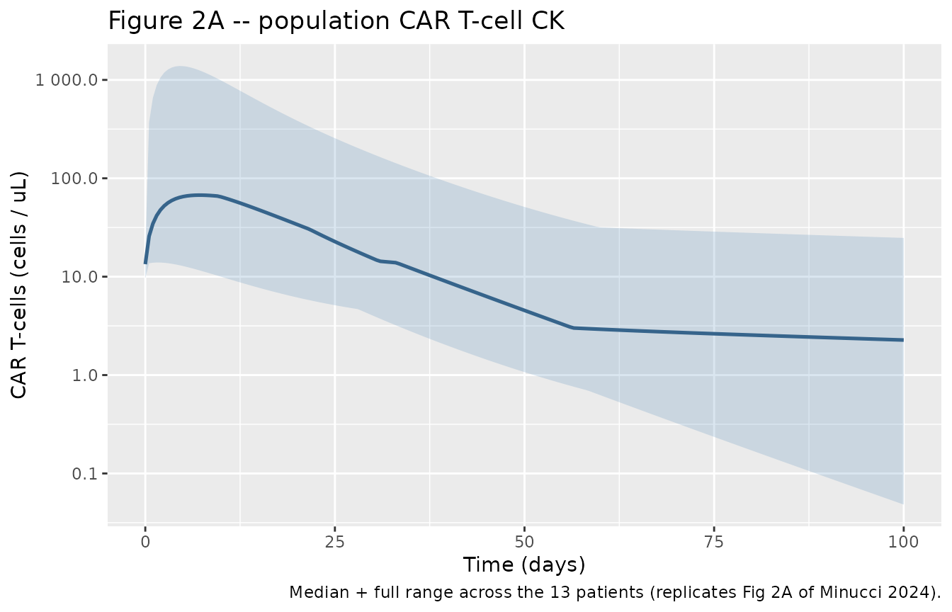
Figure 2C – individual CAR T-cell CK per patient
ggplot(sim, aes(time, pmax(CAR_perUL, 1e-4))) +
  geom_line(color = "steelblue4") +
  facet_wrap(~id_str, ncol = 4, scales = "free_y") +
  scale_y_log10(labels = scales::label_number()) +
  labs(x = "Time (days)", y = "CAR T-cells (cells / uL)",
       title = "Figure 2C -- per-patient CAR T-cell CK",
       caption = "Replicates the per-panel trajectories of Fig 2C of Minucci 2024.")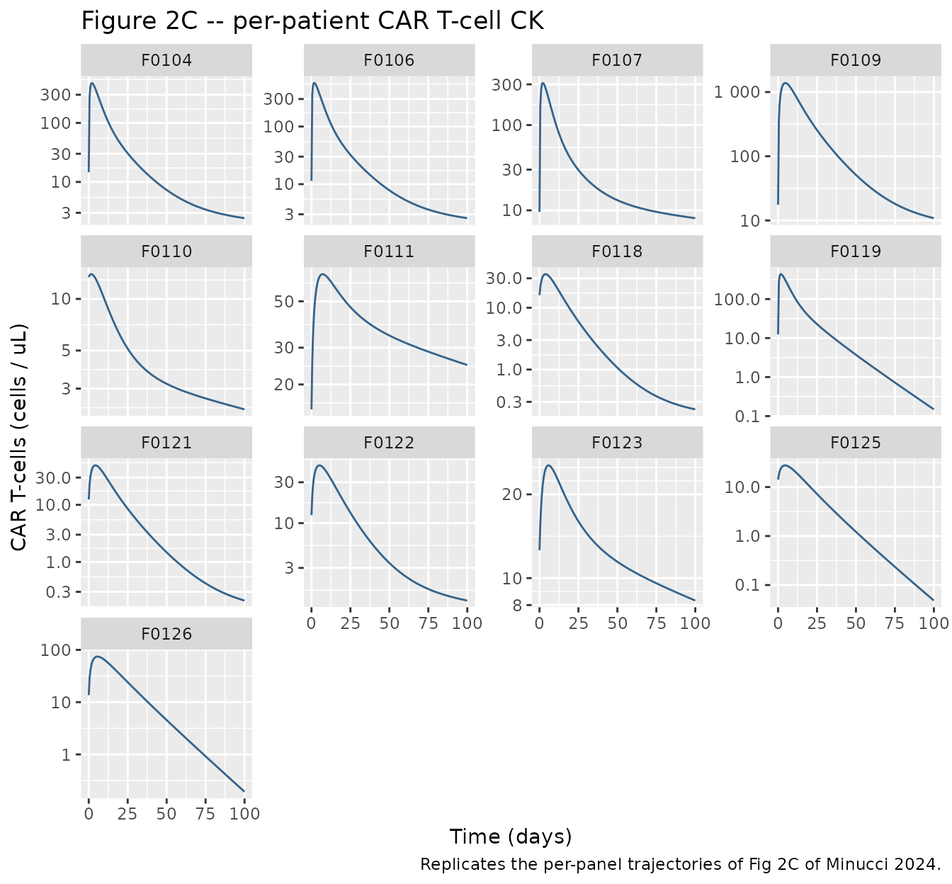
Figure 2B – B-cell aplasia trajectory
The B-cell aplasia readout is B cells as percentage of total blood lymphocytes (B_pct = 100 * tumor / (tumor + endo)). Compare against the population trend in Figure 2B of Minucci 2024.
pop_bp <- sim |>
  dplyr::group_by(time) |>
  dplyr::summarise(
    Q50 = median(B_pct, na.rm = TRUE),
    Qmax = max(B_pct, na.rm = TRUE),
    Qmin = min(B_pct, na.rm = TRUE),
    .groups = "drop"
  )

ggplot(pop_bp, aes(time, Q50)) +
  geom_ribbon(aes(ymin = Qmin, ymax = Qmax), alpha = 0.20, fill = "firebrick") +
  geom_line(color = "firebrick4", linewidth = 0.9) +
  labs(x = "Time (days)", y = "B cells (% of total lymphocytes)",
       title = "Figure 2B -- B-cell aplasia",
       caption = "Median + range across 13 patients (replicates Fig 2B of Minucci 2024).")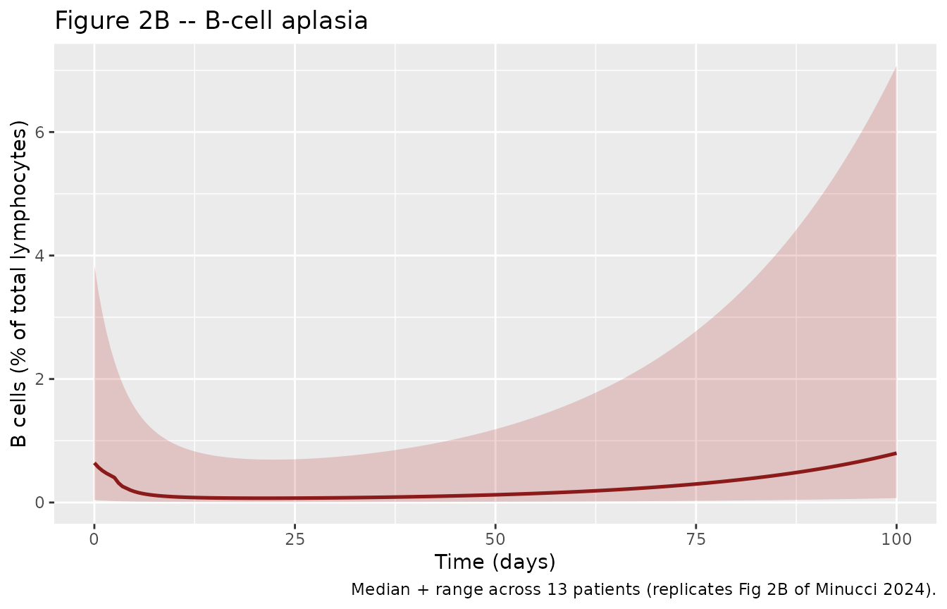
CAR T CK NCA (PKNCA)
Compute peak (Cmax), time to peak (Tmax), AUC0-inf, and terminal half-life from the simulated CAR T-cell trajectories using PKNCA. This gives a summary of the CK model’s key kinetic descriptors.
# Concentration frame -- rename CAR_perUL to log_car (nlmixr2lib convention).
sim_nca <- sim |>
  dplyr::filter(!is.na(CAR_perUL)) |>
  dplyr::select(id, id_str, time, log_car = CAR_perUL)

# Ensure a time=0 row per subject with log_car=0 (extravascular pre-dose).
sim_nca <- dplyr::bind_rows(
  sim_nca,
  sim_nca |> dplyr::distinct(id, id_str) |>
    dplyr::mutate(time = 0, log_car = 0)
) |>
  dplyr::distinct(id, id_str, time, .keep_all = TRUE) |>
  dplyr::arrange(id, id_str, time)

conc_obj <- PKNCA::PKNCAconc(sim_nca, log_car ~ time | id_str + id)

# Dose frame -- one total-CAR-dose event per subject.
dose_df <- patients_dose |>
  dplyr::transmute(id, id_str, time = 0, amt = dose_total)

dose_obj <- PKNCA::PKNCAdose(dose_df, amt ~ time | id_str + id)

intervals <- data.frame(
  start = 0, end = Inf,
  cmax = TRUE, tmax = TRUE, aucinf.obs = TRUE, half.life = TRUE
)

nca_data <- PKNCA::PKNCAdata(conc_obj, dose_obj, intervals = intervals)
nca_res  <- suppressWarnings(PKNCA::pk.nca(nca_data))
nca_res_df <- as.data.frame(nca_res)

nca_wide <- nca_res_df |>
  dplyr::select(id_str, PPTESTCD, PPORRES) |>
  tidyr::pivot_wider(names_from = PPTESTCD, values_from = PPORRES)

nca_wide |>
  dplyr::rename(
    "Patient"                 = id_str,
    "Cmax (cells/uL)"         = cmax,
    "Tmax (day)"              = tmax,
    "AUC0-inf (cells*day/uL)" = aucinf.obs,
    "t1/2 (day)"              = half.life
  ) |>
  knitr::kable(digits = 3,
caption = "Simulated per-patient CAR T-cell CK NCA (from PKNCA).")| Patient | Cmax (cells/uL) | Tmax (day) | tlast | clast.obs | lambda.z | r.squared | adj.r.squared | lambda.z.time.first | lambda.z.time.last | lambda.z.n.points | clast.pred | t1/2 (day) | span.ratio | AUC0-inf (cells*day/uL) |
|---|---|---|---|---|---|---|---|---|---|---|---|---|---|---|
| F0104 | 474.578 | 2.0 | 100 | 2.433 | 0.009 | 1 | 1 | 97.5 | 100 | 6 | 2.432 | 74.426 | 0.034 | 4937.799 |
| F0106 | 569.332 | 2.0 | 100 | 2.569 | 0.010 | 1 | 1 | 97.5 | 100 | 6 | 2.568 | 72.462 | 0.035 | 5519.909 |
| F0107 | 311.218 | 2.0 | 100 | 8.093 | 0.006 | 1 | 1 | 93.0 | 100 | 15 | 8.091 | 115.326 | 0.061 | 5236.650 |
| F0109 | 1384.205 | 4.5 | 100 | 10.852 | 0.014 | 1 | 1 | 98.0 | 100 | 5 | 10.850 | 49.520 | 0.040 | 23983.629 |
| F0110 | 13.936 | 1.5 | 100 | 2.271 | 0.006 | 1 | 1 | 81.5 | 100 | 38 | 2.269 | 120.066 | 0.154 | 855.424 |
| F0111 | 67.426 | 7.0 | 100 | 24.779 | 0.006 | 1 | 1 | 77.5 | 100 | 46 | 24.762 | 118.576 | 0.190 | 8081.463 |
| F0118 | 34.941 | 4.0 | 100 | 0.227 | 0.013 | 1 | 1 | 98.0 | 100 | 5 | 0.227 | 54.102 | 0.037 | 596.759 |
| F0119 | 434.454 | 2.0 | 100 | 0.149 | 0.064 | 1 | 1 | 48.0 | 100 | 105 | 0.146 | 10.760 | 4.833 | 3840.820 |
| F0121 | 48.970 | 4.5 | 100 | 0.211 | 0.019 | 1 | 1 | 98.0 | 100 | 5 | 0.211 | 36.690 | 0.055 | 814.484 |
| F0122 | 47.223 | 5.0 | 100 | 1.248 | 0.009 | 1 | 1 | 97.5 | 100 | 6 | 1.248 | 78.328 | 0.032 | 1169.838 |
| F0123 | 25.427 | 6.0 | 100 | 8.305 | 0.006 | 1 | 1 | 79.5 | 100 | 42 | 8.300 | 122.447 | 0.167 | 2805.137 |
| F0125 | 27.696 | 4.5 | 100 | 0.048 | 0.064 | 1 | 1 | 50.0 | 100 | 101 | 0.047 | 10.756 | 4.649 | 549.969 |
| F0126 | 74.446 | 5.5 | 100 | 0.193 | 0.064 | 1 | 1 | 33.5 | 100 | 134 | 0.189 | 10.884 | 6.110 | 1622.284 |
The above summary is simulated, not observed – Minucci 2024 does not publish a per-patient Cmax / AUC table for readers to cross-check. The paper’s Figure 2A / 2C provide the visual comparison against the individually digitised Ying 2021 data.
Peak-CAR summary vs. dose level
Sensitivity of Cmax to dose level (1e5, 1e6, 3e6 cells / kg) for a representative patient (F0104). This mirrors the “Simulations were initialized with a 1e6 cells/kg dose” language in Methods 2.4 and shows the dose-response pattern of CAR T-cell expansion.
scan_doses <- c(1e5, 1e6, 3e6)
pt_F0104   <- patients_dose |> dplyr::filter(id_str == "F0104")

build_scan_events <- function(d, id) {
  dose_total_i <- pt_F0104$BW * d
  amt_cd8_i    <- pt_F0104$fCD8Tdp * dose_total_i
  amt_cd4_i    <- (1 - pt_F0104$fCD8Tdp) * dose_total_i
  base <- tibble::tibble(
    id = id, WT = pt_F0104$BW, FCD8TDP = pt_F0104$fCD8Tdp,
    TUM_CELLS0 = pt_F0104$N0_tumorCells,
    NDIV = pt_F0104$ndiv, FMEM = pt_F0104$fmem,
    dose_per_kg = d
  )
  dplyr::bind_rows(
    base |> dplyr::mutate(time = 0, amt = amt_cd8_i,
                          cmt = "t_cd8_inf", evid = 1L),
    base |> dplyr::mutate(time = 0, amt = amt_cd4_i,
                          cmt = "t_cd4_inf", evid = 1L),
    base |> tidyr::crossing(time = seq(0, 60, by = 0.5)) |>
      dplyr::mutate(amt = NA_real_, cmt = "t_cd8_eff", evid = 0L)
  )
}

scan_events <- dplyr::bind_rows(lapply(
  seq_along(scan_doses),
  function(i) build_scan_events(scan_doses[i], id = i)
))

sim_scan <- rxode2::rxSolve(mod, events = scan_events, keep = c("dose_per_kg")) |>
  as.data.frame()
#> Warning: multi-subject simulation without without 'omega'

ggplot(sim_scan, aes(time, pmax(CAR_perUL, 1e-4),
                     color = factor(dose_per_kg))) +
  geom_line(linewidth = 0.9) +
  scale_y_log10(labels = scales::label_number()) +
  scale_color_brewer(palette = "Set1", name = "Dose (cells / kg)") +
  labs(x = "Time (days)", y = "CAR T-cells (cells / uL)",
       title = "Dose-response of CAR T-cell expansion (patient F0104)",
       caption = "One-at-a-time dose scan; other parameters held at F0104 fitted values.")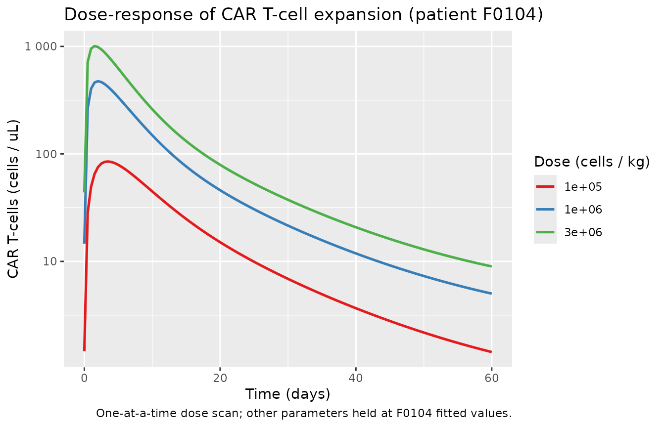
Assumptions and deviations
QSS reduction of the receptor-binding sub-model. Minucci 2024’s original model tracks free and CD19-bound CAR receptors on each T-cell phenotype (14 CAR receptor states) plus a transient activated-cell compartment T_act. With CAR:CD19 binding rates ~86/day and cellular rates 0.005-0.3/day, quasi-steady-state gives f_bound = [CD19] / (K_D + [CD19]) uniformly across all CAR compartments. T_act relaxes on a ~5.4 h timescale (much shorter than any observed transient) and its amplification factor 2^ndiv is folded into the T_inf -> T_eff transfer via the fast-T_act QSS. The observed cell populations, tumor burden, and B-cell aplasia trajectories are preserved. The full explicit 25-state model is available in principle but was reduced here for numerical stability and vignette-render time; see the file header block-comment in the model file for the mapping.
Endogenous lymphocyte concentration. Methods 2.3.1 of the paper reports 10^9 per L but the supplementary Table S1 (
params-case-study-final) lists 5e8 per L; the Table S1 value is used here because the final parameter sheet takes precedence over the Methods text. The final case-study simulations use Table S1 values.CD19 receptors per cell. Methods 2.3.1 reports 5000 per B cell and Table S1 lists
mAgperCell = 5000and alsoRPC_CD19 = 15877, both described as “Antigen expression level”. Only mAgperCell = 5000 is documented in the paper text; the second entry is unexplained. The extraction uses 5000 (aligns with paper text and GSA nominal), and documents the duplicate as a possible transcription artefact of the supplement’s parameter export.Tumor carrying capacity
Nmax_tumor = 7e12is estimated (Methods 2.3.1, Press 1993) but does not appear in the paper’s stated Tumor ODE (Methods 2.3, pure exponential minus killing). Within the 100-day simulation window Tumor stays well belowNmax_tumorfor all patients in Table S1, so omission has no effect on the simulated trajectories.Residual error. Minucci 2024 fitted each patient individually with trust-region optimisation and did not publish a population residual- error model. A nominal fixed
addSd = 0.1onlog(CAR_perUL)is retained so the model has a well-formed error line for nlmixr2 UI, but it is zeroed withrxode2::zeroRe(mod)throughout this vignette. The vignette’s outputs are typical-value (deterministic) predictions, not VPCs.Newly registered covariates.
FCD8TDP(drug-product CD8 fraction),TUM_CELLS0(initial tumor cells),NDIV(T-cell expansion factor), andFMEM(fraction of effector T-cells that become memory) had no canonical entries when this model was first drafted. All four were ratified by the maintainers and added toinst/references/covariate-columns.mdasscope: specificcanonicals in the Oncology section, socheckModelConventions()now reports zero issues for this model.TUM_CELLS0is deliberately kept distinct from the existingTUMSZ/TUM_SLD/TUM_VOLfamily, which carries length- and volume-based tumor measures, because this column’s currency is an absolute malignant-cell count with no source-defined conversion to a length or volume.Three of the four new covariates are fit outputs, not measurements.
TUM_CELLS0,NDIV, andFMEMwere obtained by per-patient trust-region optimisation against each subject’s own CAR T-cell cellular-kinetic trajectory, so they are model inputs rather than independently observable patient characteristics. Several values sit exactly on the optimiser’s bounds –TUM_CELLS0at 1e5 (F0109, F0110, F0111, F0123) and 1e7 (F0104, F0106, F0107, F0118, F0119), andFMEMat the 0.1 upper bound (F0110, F0111, F0123) with three further patients numerically indistinguishable from zero (F0119, F0125, F0126). Treat these as identifiability-limited: the paper reports no uncertainty on them, and the model reproduces the published trajectories rather than establishing that the values are uniquely determined.FCD8TDPis the exception – it is a measured property of the manufactured drug product, taken from the per-patient CD4:CD8 ratios reported in Ying 2021.Non-canonical compartment names. The six CAR T-cell state compartments (
t_cd8_inf,t_cd8_eff,t_cd8_mem,t_cd4_inf,t_cd4_eff,t_cd4_mem) and the endogenous-lymphocyte compartment (endo) are not registered inR/conventions.R.checkModelConventions()flags them as warnings. If further CAR T-cell / immunology QSP models are extracted, adding these to the compartment register is warranted.Original observed data. Ying et al. 2021’s patient-level CK and B-cell aplasia trajectories are not shipped with either paper. Minucci 2024 obtained them by digitising Figure 2 of Ying 2021 with WebPlotDigitizer; only 6 of the 13 patients had B-cell aplasia trajectories distinguishable enough to digitise. This vignette therefore validates the model against the paper’s Figure 2 visualisation rather than against the raw source data.