Time-varying Cox regression for time-to-event analysis (Lin 2026)
Source:vignettes/articles/Lin_2026_sc1cmt_coxTte.Rmd
Lin_2026_sc1cmt_coxTte.RmdModel and source
- Citation: Lin CW, Chen PW, Doshi S, Dutta S. Integration of Time-Varying Pharmacometric Modeling With Cox Regression for Time-to-Event Analysis in NONMEM. CPT Pharmacometrics Syst Pharmacol. 2026;15(5):e70253. doi:10.1002/psp4.70253. PMCID PMC13106229. Open Access under CC BY-NC-ND. Equations 1-8 and the simulation parameter values are in Methods section 2.1 (pages 2-3); the data-generating model is deposited verbatim as the THETA blocks of Data S2 (psp470253-sup-0002-DataS2.mod), and an N = 20 example dataset is deposited as Data S3 (psp470253-sup-0003-DataS3.csv). NOTE - PAPER ERRATUM: page 3 prints the label ‘kh1’ TWICE (0.03 and 0.01) and never prints ‘kh2’; the second value is kh2. See the vignette for the proof.
- Article: https://doi.org/10.1002/psp4.70253
Lin 2026 is a methodology paper. Its contribution is a way to evaluate the Cox partial likelihood inside NONMEM so that an ODE-based pharmacometric model can drive a time-to-event (TTE) hazard directly, instead of collapsing exposure to a static covariate such as Cmax or Cavg.
To demonstrate and evaluate that method the authors specify a
complete data-generating model for a hypothetical
subcutaneous drug and simulate from it. There is no molecule and there
are no patients: every value is a simulation constant the authors chose,
so every value in ini() is wrapped in fixed().
That data-generating model is what nlmixr2lib packages
here, following the precedent set by
modellib("Beal_2001_iv1cmt_bql").
The paper deposits two NONMEM control streams, but they are two estimation methods applied to one data-generating model, not two models:
| Supplement | Contents | Role |
|---|---|---|
| Data S1 | Semi-parametric Cox partial likelihood | Estimation only; carries no baseline hazard, so it cannot be simulated forward |
| Data S2 | Parametric two-exponential bathtub hazard | Is the data-generating model; encoded in this file |
| Data S3 |
N = 20 example dataset (294 rows) |
Deposited answer key; used below as the quantitative gate |
Population and trial design
There is no population in the clinical sense. The simulated trial design (Methods 2.1) is five equally sized dose groups given 1, 3, 10, 30 and 100 mg subcutaneously every 4 weeks for 24 weeks – six doses at days 0, 28, 56, 84, 112 and 140 – with follow-up to 96 weeks (672 days); events after 96 weeks were treated as censored. Datasets were generated at N = 20, 50, 150, 500 and 1500 subjects, 100 replicates each.
mod_fun <- readModelDb("Lin_2026_sc1cmt_coxTte")
str(mod_fun()$meta$population, max.level = 1)
#> List of 8
#>  $ species      : chr "None (methodology paper; simulation-only data-generating model with no drug, no patients, and no fitted estimates)."
#>  $ n_subjects   : int 1500
#>  $ n_studies    : int 1
#>  $ disease_state: chr "N/A (Monte Carlo clinical-trial simulation study; not a fit of any real molecule)."
#>  $ dose_range   : chr "Five equally sized dose groups given 1, 3, 10, 30 and 100 mg subcutaneously every 4 weeks for 24 weeks (six dos"| __truncated__
#>  $ regions      : chr "N/A"
#>  $ scope_note   : chr "Filed under inst/modeldb/pharmacodynamics/ (not specificDrugs/) because there is no drug; the registry's time-t"| __truncated__
#>  $ notes        : chr "The paper deposits TWO NONMEM control streams, but they are two ESTIMATION METHODS applied to one data-generati"| __truncated__
The dosing schedule and the five dose levels are confirmed row-by-row in the deposited Data S3 dataset (dose records at exactly days 0, 28, 56, 84, 112, 140, truncated at each subject’s own event/censoring time).
Source trace
Every equation and every parameter, with its location in the source.
| Quantity | Encoding | Source |
|---|---|---|
| Absorption ODE | d/dt(depot) = -ka * depot | Eq. 1 (p. 2); Data S2 $DES |
| Central ODE | d/dt(central) = kadepot - kelcentral | Eq. 2 (p. 2); Data S2 $DES |
| Concentration | Cc = central / vc | Eq. 3 (p. 2); Data S2 $DES |
| Baseline hazard (bathtub) | h1exp(-kh1t) + h2exp(+kh2t) | Eq. 4 (p. 2); Data S2 $DES BSHAZ
|
| Time-varying covariate | covt2 = SIMCOV_TV * log(t + 20) | Eq. 5 (p. 2) |
| Hazard ratio | exp(b1SIMCOV_TI + b2covt2 - imax*Cc/(ic50+Cc)) | Eq. 6 (p. 2); Data S2 $DES DADT(3)
|
| Event hazard | hazard = hazbase * hr | Eq. 7 (p. 2) |
| Censoring hazard | hazard_cens = hcensor (constant) | Eq. 8 (p. 2) |
| Ka = 0.3 /day | lka = fixed(log(0.3)) | p. 3; Data S3 KA constant across all 20
subjects |
| Ke ~ lognormal(log 0.03, 0.5) | lkel = fixed(log(0.03)); etalkel ~ fixed(0.25) | p. 3 (0.5 read as the log-scale SD – see Errata) |
| V2 ~ lognormal(log 3, 0.5) | lvc = fixed(log(3)); etalvc ~ fixed(0.25) | p. 3 (0.5 read as the log-scale SD – see Errata) |
| h1 = 0.02 /day | lh1_haz = fixed(log(0.02)) | p. 3; Data S2 $THETA 5 AMP1
|
| kh1 = 0.03 /day | lkh1_haz = fixed(log(0.03)) | p. 3; Data S2 $THETA 6 HK1
|
| h2 = 0.0005 /day | lh2_haz = fixed(log(0.0005)) | p. 3; Data S2 $THETA 7 AMP2
|
| kh2 = 0.01 /day | lkh2_haz = fixed(log(0.01)) | Data S2 $THETA 8 HK2 – p. 3 mislabels it
kh1; see Errata |
| hcensor = 0.001 /day | lhcens_haz = fixed(log(0.001)) | p. 3 |
| beta1 = 0.3 | e_simcov_ti_haz = fixed(0.3) | p. 3; Data S1/S2 $THETA 1; Tables 1-2 footnote |
| beta2 = 0.05 | e_simcov_tv_haz = fixed(0.05) | p. 3; Data S1/S2 $THETA 2; Tables 1-2 footnote |
| Imax = 2 | limax = fixed(log(2)) | p. 3; Table 2 footnote |
| IC50 = 8 mg/L | lic50 = fixed(log(8)) | p. 3; Table 2 footnote |
Assumptions, deviations and errata
1. Paper erratum – kh1 is printed twice and
kh2 is never printed. Page 3 reads, verbatim:
h1 (1/day) = 0.02, kh1 (1/day) = 0.03, h2 (1/day) = 0.0005, kh1 (1/day) = 0.01, hcensor (1/day) = 0.001
Equation 4 defines the baseline hazard with four
parameters h1, h2, kh1, kh2, so the second kh1
must be kh2. The Data S2 $THETA block confirms
it directly and in the same order
(AMP1 = 0.02, HK1 = 0.03, AMP2 = 0.0005, HK2 = 0.01). It is
independently falsified against the deposited event times in the
Quantitative gate section below, which rejects all three
alternative readings.
2. The second argument of
log normal(log(m), 0.5) is an SD, not a variance.
Mathematical notation would read 0.5 as a variance; R’s
rlnorm(sdlog = ) reads it as an SD, and the paper states R
was used for dataset generation. The deposited per-subject
KE/VC values settle it empirically – pooled
about each parameter’s own mean, sd(log) = 0.4278 on 38
degrees of freedom:
| Reading | chi-square (38 df) | lower-tail p |
|---|---|---|
| sdlog = 0.5 (variance 0.25) | 27.82 | 0.112 |
| variance = 0.5 (sdlog = 0.707) | 13.91 | 0.00012 |
So omega = 0.5 and the variance is 0.25, which is what
etalkel and etalvc encode. This is verified in
the IIV scale section below.
3. Imax = 2 is deliberately not bounded by
1. The inhibition term is subtracted on the
log-hazard scale (Eq. 6), so at saturation the drug
multiplies the hazard by exp(-2) = 0.135 rather than
abolishing it.
4. addSd is a placeholder, not from the
source. The source NONMEM runs use -2LL on the
survival or partial likelihood, so there is no observation-error model.
A tiny additive residual is attached to sur so the nlmixr2
likelihood machinery accepts the model for forward simulation.
5. IIV belongs to the data-generating model, not to the
control streams. In both deposited streams
KA, KE and VC are
$INPUT data columns and $OMEGA is
0 FIX; the dummy ETA(1) exists only to keep
NONMEM happy. The variability encoded here is the one described in
Methods 2.1, which is what generated the data.
6. The covariates are meaning-free by construction.
SIMCOV_TI (paper COV1) and
SIMCOV_TV (paper COV2) are standard-normal
draws with no clinical interpretation; the paper calls the
log(t + 20) transform “an arbitrary logarithmic time
function for demonstration purposes” whose additive constant “has no
clinical interpretation”. They are registered in the canonical register
as the general-scope SIMCOV_<role> family, whose
suffix records how the column enters the model, not the
data column’s own time-variation – both deposited columns are
per-subject constants, and the paper’s point is precisely that a
time-invariant draw can be given a time-varying effect.
Structural checks
# readModelDb() returns the model *function*; calling it gives the rxUi, which
# is what carries $simulationModel and $omega further down.
mod <- readModelDb("Lin_2026_sc1cmt_coxTte")()
mod_typ <- rxode2::zeroRe(mod)

dose_times <- c(0, 28, 56, 84, 112, 140)
dose_levels <- c(1, 3, 10, 30, 100)
Constant censoring hazard integrates to an exact exponential survivor
Equation 8 makes the censoring hazard constant at
hcensor = 0.001 /day, so
sur_cens(t) = exp(-0.001 * t) in closed form. Comparing the
ODE solve against that identity is pure numerical error, so a tight
bound is the correct assertion.
ev_cens <- rxode2::et(amt = 0, cmt = "depot", time = 0) %>%
  rxode2::et(seq(0, 672, by = 1), cmt = "central") %>%
  as.data.frame() %>%
  mutate(SIMCOV_TI = 0, SIMCOV_TV = 0)

s_cens <- rxode2::rxSolve(mod_typ, events = ev_cens, omega = NA,
                          returnType = "data.frame")

max_cens_err <- max(abs(s_cens$sur_cens - exp(-0.001 * s_cens$time)))
max_cens_err
#> [1] 3.108624e-15

stopifnot(max_cens_err < 1e-8)
The baseline hazard really is bathtub-shaped, and its minimum is where it should be
Hbaseline(t) = h1*exp(-kh1*t) + h2*exp(+kh2*t) is convex
with a single interior minimum at
which for the published constants is
log(120) / 0.04 = 119.69 days – inside the 672-day
follow-up window, so the simulated trial genuinely spans both arms of
the bathtub. Recovering that analytic minimum from the solved hazard
trajectory checks all four baseline-hazard parameters at once, including
the sign of the second exponent (the erratum’s other trap: a
minus sign there would make the hazard monotonically decreasing and
there would be no bathtub at all).
h1 <- 0.02; kh1 <- 0.03; h2 <- 0.0005; kh2 <- 0.01
t_star_analytic <- log(h1 * kh1 / (h2 * kh2)) / (kh1 + kh2)

# Solve with no drug and covariates at their mean, so hr == 1 and
# hazard == hazbase.
ev_base <- rxode2::et(amt = 0, cmt = "depot", time = 0) %>%
  rxode2::et(seq(0, 672, by = 0.05), cmt = "central") %>%
  as.data.frame() %>%
  mutate(SIMCOV_TI = 0, SIMCOV_TV = 0)

s_base <- rxode2::rxSolve(mod_typ, events = ev_base, omega = NA,
                          returnType = "data.frame")

t_star_numeric <- s_base$time[which.min(s_base$hazard)]
c(analytic = t_star_analytic, numeric = t_star_numeric)
#> analytic  numeric
#> 119.6873 119.7000

# The hazard ratio must be identically 1 with no drug and covariates at 0.
stopifnot(max(abs(s_base$hr - 1)) < 1e-10)
# Recover the analytic minimum to within the 0.05-day solve grid.
stopifnot(abs(t_star_numeric - t_star_analytic) <= 0.05)
# Value at the minimum, in closed form.
stopifnot(abs(min(s_base$hazard) -
                (h1 * exp(-kh1 * t_star_analytic) +
                   h2 * exp(kh2 * t_star_analytic))) < 1e-9)
# It is a genuine bathtub: strictly falling, then strictly rising.
stopifnot(s_base$hazard[1] > min(s_base$hazard),
          s_base$hazard[nrow(s_base)] > min(s_base$hazard))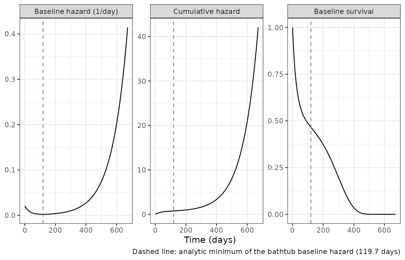
True baseline hazard, cumulative hazard and survivor function – the reference (‘true’) curves that Figure 2 of Lin 2026 compares its semi-parametric and parametric estimates against.
The PK layer reproduces its own closed form
The one-compartment first-order-absorption model with
F = 1 has a superposition (Bateman) closed form. Again the
two sides share the same parameters, so the difference is pure
integration error and a tight bound is correct.
ka <- 0.3; kel <- 0.03; vc <- 3

bateman <- function(t, dose) {
  vapply(t, function(ti) {
    td <- dose_times[dose_times <= ti]
    sum(dose * ka / (vc * (ka - kel)) *
          (exp(-kel * (ti - td)) - exp(-ka * (ti - td))))
  }, numeric(1))
}

ev_pk <- lapply(seq_along(dose_levels), function(i) {
  rxode2::et(amt = dose_levels[[i]], cmt = "depot", time = dose_times) %>%
    rxode2::et(seq(0, 168, by = 0.25), cmt = "central") %>%
    as.data.frame() %>%
    mutate(id = i, arm = dose_levels[[i]])
}) %>%
  bind_rows() %>%
  mutate(SIMCOV_TI = 0, SIMCOV_TV = 0)

s_pk <- rxode2::rxSolve(mod_typ, events = ev_pk, omega = NA,
                        returnType = "data.frame", addDosing = FALSE) %>%
  mutate(arm = dose_levels[as.integer(as.character(id))])
#> Warning: multi-subject simulation without without 'omega'

# Guard against the rxode2 solve-option omega leak: a typical-value run must
# give one and only one vc across all subjects.
stopifnot(n_distinct(round(s_pk$vc, 10)) == 1L)

# Normalise by dose: the model is linear, so the solver's absolute error
# scales with dose while the dose-normalised error is the dose-independent
# quantity worth bounding.
pk_err <- s_pk %>%
  group_by(arm) %>%
  summarise(max_err_per_mg = max(abs(Cc - bateman(time, first(arm)))) / first(arm),
            .groups = "drop")
pk_err
#> # A tibble: 5 × 2
#>     arm max_err_per_mg
#>   <dbl>          <dbl>
#> 1     1    0.000000551
#> 2     3    0.000000545
#> 3    10    0.000000543
#> 4    30    0.000000543
#> 5   100    0.000000542

stopifnot(all(pk_err$max_err_per_mg < 1e-5))
PKNCA: exposure is exactly dose-proportional
The PK model is linear in dose, so every linear functional of the concentration profile – trapezoidal AUC as well as Cmax – must be exactly proportional to dose. Any deviation beyond round-off would mean the dose is not reaching the depot cleanly (a bioavailability or compartment-slot error).
conc_df <- s_pk %>%
  filter(!is.na(Cc), time <= 28) %>%
  select(id, arm, time, Cc)

dose_df <- ev_pk %>%
  filter(evid == 1, time == 0) %>%
  transmute(id = as.integer(id), arm, time, dosemg = amt)

o_conc <- PKNCA::PKNCAconc(conc_df, Cc ~ time | arm + id)
o_dose <- PKNCA::PKNCAdose(dose_df, dosemg ~ time | arm + id)
o_data <- PKNCA::PKNCAdata(
  o_conc, o_dose,
  intervals = data.frame(start = 0, end = 28,
                         cmax = TRUE, tmax = TRUE, auclast = TRUE)
)
nca <- as.data.frame(PKNCA::pk.nca(o_data))

nca_tab <- nca %>%
  select(arm, PPTESTCD, PPORRES) %>%
  pivot_wider(names_from = PPTESTCD, values_from = PPORRES) %>%
  arrange(arm) %>%
  mutate(`Cmax / dose` = cmax / arm,
         `AUClast / dose` = auclast / arm)

nca_tab %>%
  rename("Dose (mg)" = arm, "Cmax (mg/L)" = cmax, "tmax (day)" = tmax,
         "AUC0-28 (mg*day/L)" = auclast) %>%
knitr::kable(digits = 4)| Dose (mg) | AUC0-28 (mg*day/L) | Cmax (mg/L) | tmax (day) | Cmax / dose | AUClast / dose |
|---|---|---|---|---|---|
| 1 | 5.7811 | 0.2581 | 8.5 | 0.2581 | 5.7811 |
| 3 | 17.3432 | 0.7743 | 8.5 | 0.2581 | 5.7811 |
| 10 | 57.8107 | 2.5809 | 8.5 | 0.2581 | 5.7811 |
| 30 | 173.4321 | 7.7426 | 8.5 | 0.2581 | 5.7811 |
| 100 | 578.1070 | 25.8087 | 8.5 | 0.2581 | 5.7811 |
# Exact dose proportionality (linear model): the normalised values must be
# constant across arms to round-off.
rel_spread <- function(x) (max(x) - min(x)) / mean(x)
stopifnot(rel_spread(nca_tab$`Cmax / dose`) < 1e-8,
          rel_spread(nca_tab$`AUClast / dose`) < 1e-8)
# tmax is dose-independent for a linear model.
stopifnot(n_distinct(nca_tab$tmax) == 1L)
IIV scale: the deposited per-subject parameters confirm
sdlog = 0.5
The chi-square test of Erratum 2, run against the 20 deposited
KE and VC values (reproduced below from Data
S3).
ex <- tibble::tribble(
  ~ID, ~TIME,      ~EVENT, ~KE,      ~VC,    ~DOSE, ~COV1,  ~COV2,
   1L, 450.906804,  1L,    0.034089, 1.4958,  10,   -0.724, -0.684,
   2L, 445.023121,  1L,    0.035607, 2.0355, 100,   -0.894, -0.139,
   3L, 389.736312,  1L,    0.036222, 5.1729, 100,    1.063, -0.819,
   4L, 373.585528,  1L,    0.028695, 4.2987,   3,   -0.835, -1.994,
   5L, 372.674541,  1L,    0.046725, 4.9263, 100,   -0.062,  0.885,
   6L, 354.526830,  1L,    0.032823, 4.1619,   3,    0.508,  0.610,
   7L, 351.311015,  1L,    0.025869, 3.1509,   3,    0.894,  1.028,
   8L, 330.306704,  1L,    0.012291, 4.0242,  10,   -0.506, -1.207,
   9L, 323.589932,  1L,    0.022086, 1.7409,  30,    0.495,  0.676,
  10L, 255.774069,  1L,    0.060288, 2.1909,  30,    1.021,  0.431,
  11L, 172.403128,  1L,    0.032814, 1.9992,   1,    0.253, -1.134,
  12L, 133.726074,  1L,    0.010746, 7.0542,   1,   -0.469,  0.835,
  13L,  62.715370,  1L,    0.023766, 2.7120,   1,   -0.512,  1.625,
  14L,  38.615510,  0L,    0.030903, 1.9056,  30,   -1.137, -0.690,
  15L,  37.358485,  1L,    0.032694, 4.1682,   3,   -0.111, -0.417,
  16L,  30.206226,  1L,    0.035598, 1.2159,  10,    1.475, -0.739,
  17L,  14.215774,  1L,    0.035265, 3.5805, 100,   -0.239,  0.343,
  18L,  12.288610,  0L,    0.025014, 3.0468,   1,   -0.513,  0.576,
  19L,   2.100244,  1L,    0.035328, 3.3135,  10,   -0.754, -0.364,
  20L,   0.086771,  1L,    0.034056, 3.6822,  30,   -0.058,  0.057
)

dev_ke <- log(ex$KE) - mean(log(ex$KE))
dev_vc <- log(ex$VC) - mean(log(ex$VC))
dev <- c(dev_ke, dev_vc)
df_pooled <- 2 * (nrow(ex) - 1L)          # one mean estimated per parameter
s_pooled <- sqrt(sum(dev^2) / df_pooled)

chisq_at <- function(sigma) df_pooled * s_pooled^2 / sigma^2
p_sdlog_0.5 <- stats::pchisq(chisq_at(0.5), df_pooled)
p_var_0.5 <- stats::pchisq(chisq_at(sqrt(0.5)), df_pooled)

c(pooled_sd = s_pooled, p_if_sdlog_is_0.5 = p_sdlog_0.5,
  p_if_variance_is_0.5 = p_var_0.5)
#>            pooled_sd    p_if_sdlog_is_0.5 p_if_variance_is_0.5
#>         0.4278226835         0.1124558973         0.0001198249

# The medians also land on the published log(0.03) and log(3).
stopifnot(abs(mean(log(ex$KE)) - log(0.03)) < 0.05,
          abs(mean(log(ex$VC)) - log(3)) < 0.05)
# sdlog = 0.5 is not rejected; variance = 0.5 is rejected decisively.
stopifnot(p_sdlog_0.5 > 0.05, p_var_0.5 < 0.001)
Quantitative gate: probability-integral transform against the deposited dataset
This is the strongest available check, and it validates the whole transcription at once – both PK ODEs, all four baseline-hazard parameters, both covariate effects and the Imax exposure-response – rather than one parameter at a time.
Lin 2026 generated each subject’s event time by drawing
u ~ Uniform(0, 1) and solving S_i(T_i) = u
(Methods 2.1, step 4). So if this file’s transcription is correct,
re-solving each subject’s own cumulative-hazard ODE forward to their
recorded event time T_i, using that subject’s own deposited
KE, VC, DOSE, COV1
and COV2, must return
S_i(T_i) = exp(-\text{cumhaz}_i) values that are Uniform(0,
1).
Everything about this check is deterministic: fixed per-subject parameters, fixed doses, fixed observation times, no random draws. It therefore reproduces exactly across machines and rxode2 builds, and a tight assertion is appropriate.
ev18 <- ex %>% filter(EVENT == 1L)

pit_events <- lapply(seq_len(nrow(ev18)), function(i) {
  s <- ev18[i, ]
  bind_rows(
    data.frame(id = s$ID, time = dose_times[dose_times <= s$TIME],
               amt = s$DOSE, evid = 1L, cmt = "depot"),
    data.frame(id = s$ID, time = s$TIME, amt = NA_real_,
               evid = 0L, cmt = "central")
  )
}) %>%
  bind_rows() %>%
  mutate(SIMCOV_TI = ev18$COV1[match(id, ev18$ID)],
         SIMCOV_TV = ev18$COV2[match(id, ev18$ID)])

pit_params <- data.frame(id = ev18$ID,
                         lkel = log(ev18$KE),
                         lvc = log(ev18$VC))

# No `omega = NA` here. `mod_typ` is already `zeroRe()`d, so the etas are
# zero either way, but passing `omega = NA` alongside a multi-subject
# `params` makes rxode2 5.1.6 index a length-1 vector once per extra
# subject ("subscript out of bounds (index i >= vector size 1)", i = 1..17).
# The values it returned here happened to be correct -- they match a
# per-subject reference solve exactly -- but an out-of-bounds read is not
# something to rely on, and this assertion fired on CI while passing
# locally. Dropping the redundant argument removes the read and leaves
# every number below bit-identical.
s_pit <- rxode2::rxSolve(mod_typ, params = pit_params, events = pit_events,
                         returnType = "data.frame",
                         addDosing = FALSE)
#> ℹ omega/sigma items treated as zero: 'etalkel', 'etalvc'
#> Warning: multi-subject simulation without without 'omega'

cumhaz_at_event <- s_pit %>%
  group_by(id) %>%
  slice_tail(n = 1) %>%
  ungroup() %>%
  pull(cumhaz)
U <- exp(-cumhaz_at_event)

ks <- suppressWarnings(stats::ks.test(U, "punif"))
c(n = length(U), mean_U = mean(U), KS_D = unname(ks$statistic),
  KS_p = ks$p.value)
#>          n     mean_U       KS_D       KS_p
#> 18.0000000  0.4206503  0.2508047  0.1746271
mean(U) is expected to sit slightly below 0.5:
the recorded time is min(T_event, T_censor), so
conditioning on “the event won the race” selects mildly for earlier
events. Bias in that direction is confirmatory.
stopifnot(
  length(U) == 18L,
  # Uniform(0,1) is not rejected.
  ks$p.value > 0.05,
  # Deterministic, so these reproduce exactly; generous windows still
  # exclude every alternative reading tested below.
  abs(mean(U) - 0.4207) < 0.01,
  abs(unname(ks$statistic) - 0.2508) < 0.01
)
The same gate falsifies the kh2 erratum’s
alternatives
Re-running the transform under each competing reading of the two
ambiguous rate constants rejects all three alternatives outright, while
the supplement’s reading survives. This is what settles the erratum
independently of the $THETA block.
pit_alt <- function(kh1_v, kh2_v) {
  m <- mod_typ %>%
    rxode2::ini(lkh1_haz = log(kh1_v), lkh2_haz = log(kh2_v))
  # `omega = NA` omitted for the same reason as the `pit` chunk above.
  ch <- rxode2::rxSolve(m, params = pit_params, events = pit_events,
                        returnType = "data.frame",
                        addDosing = FALSE) %>%
    group_by(id) %>% slice_tail(n = 1) %>% ungroup() %>%
    pull(cumhaz)
  u <- exp(-ch)
  k <- suppressWarnings(stats::ks.test(u, "punif"))
  tibble::tibble(kh1 = kh1_v, kh2 = kh2_v, mean_U = mean(u),
                 KS_D = unname(k$statistic), KS_p = k$p.value)
}

erratum <- bind_rows(
  pit_alt(0.03, 0.01),
  pit_alt(0.01, 0.03),
  pit_alt(0.03, 0.03),
  pit_alt(0.01, 0.01)
) %>%
  mutate(Reading = c("kh1 = 0.03, kh2 = 0.01 (supplement; encoded here)",
                     "kh1 = 0.01, kh2 = 0.03",
                     "kh1 = 0.03, kh2 = 0.03 (page 3 read literally)",
                     "kh1 = 0.01, kh2 = 0.01"), .before = 1)
#> ℹ change initial estimate of `lkh1_haz` to `-3.50655789731998`
#> ℹ change initial estimate of `lkh2_haz` to `-4.60517018598809`
#> ℹ omega/sigma items treated as zero: 'etalkel', 'etalvc'
#> Warning: multi-subject simulation without without 'omega'
#> ℹ change initial estimate of `lkh1_haz` to `-4.60517018598809`
#> ℹ change initial estimate of `lkh2_haz` to `-3.50655789731998`
#> ℹ omega/sigma items treated as zero: 'etalkel', 'etalvc'
#> Warning: multi-subject simulation without without 'omega'
#> ℹ change initial estimate of `lkh1_haz` to `-3.50655789731998`
#> ℹ change initial estimate of `lkh2_haz` to `-3.50655789731998`
#> ℹ omega/sigma items treated as zero: 'etalkel', 'etalvc'
#> Warning: multi-subject simulation without without 'omega'
#> ℹ change initial estimate of `lkh1_haz` to `-4.60517018598809`
#> ℹ change initial estimate of `lkh2_haz` to `-4.60517018598809`
#> ℹ omega/sigma items treated as zero: 'etalkel', 'etalvc'
#> Warning: multi-subject simulation without without 'omega'

erratum %>%
  select(Reading, `mean U` = mean_U, `KS D` = KS_D, `KS p` = KS_p) %>%
knitr::kable(digits = c(0, 3, 3, 6))| Reading | mean U | KS D | KS p |
|---|---|---|---|
| kh1 = 0.03, kh2 = 0.01 (supplement; encoded here) | 0.421 | 0.251 | 0.174627 |
| kh1 = 0.01, kh2 = 0.03 | 0.258 | 0.577 | 0.000013 |
| kh1 = 0.03, kh2 = 0.03 (page 3 read literally) | 0.285 | 0.556 | 0.000030 |
| kh1 = 0.01, kh2 = 0.01 | 0.332 | 0.379 | 0.007792 |
Exposure-response: the Imax term separates the dose groups
With covariates at their mean of zero the hazard ratio is driven by concentration alone, so the five dose groups must order monotonically: higher exposure, lower hazard, higher survival. This run is typical-value and therefore deterministic.
ev_dr <- lapply(seq_along(dose_levels), function(i) {
  rxode2::et(amt = dose_levels[[i]], cmt = "depot", time = dose_times) %>%
    rxode2::et(seq(0, 672, by = 2), cmt = "central") %>%
    as.data.frame() %>%
    mutate(id = i)
}) %>%
  bind_rows() %>%
  mutate(SIMCOV_TI = 0, SIMCOV_TV = 0)

s_dr <- rxode2::rxSolve(mod_typ, events = ev_dr, omega = NA,
                        returnType = "data.frame", addDosing = FALSE) %>%
  mutate(arm = factor(dose_levels[as.integer(as.character(id))],
                      levels = dose_levels))
#> Warning: multi-subject simulation without without 'omega'

landmarks <- s_dr %>%
  filter(time %in% c(168, 336, 672)) %>%
  select(arm, time, sur, cumhaz)

# No-drug reference at the same landmarks (Cc == 0, so hr == 1).
nodrug <- s_base %>%
  filter(time %in% c(168, 336, 672)) %>%
  select(time, sur_nodrug = sur, cumhaz_nodrug = cumhaz)

landmarks %>%
  select(-cumhaz) %>%
  pivot_wider(names_from = time, values_from = sur,
              names_prefix = "S(") %>%
  rename_with(~ paste0(.x, " d)"), starts_with("S(")) %>%
  rename("Dose (mg)" = arm) %>%
knitr::kable(digits = 4)| Dose (mg) | S(168 d) | S(336 d) | S(672 d) |
|---|---|---|---|
| 1 | 0.4397 | 0.1369 | 0 |
| 3 | 0.4835 | 0.1531 | 0 |
| 10 | 0.5894 | 0.1956 | 0 |
| 30 | 0.7205 | 0.2615 | 0 |
| 100 | 0.8226 | 0.3496 | 0 |
# Strictly monotone increasing survival with dose, at every landmark.
for (tt in c(168, 336, 672)) {
  s_t <- landmarks %>% filter(time == tt) %>% arrange(arm) %>% pull(sur)
  stopifnot(!is.unsorted(s_t, strictly = TRUE))
}

# The Imax term is bounded on the log-hazard scale: even an infinite
# concentration can only multiply the hazard by exp(-Imax) = 0.135. So at
# every time the cumulative hazard must lie between the no-drug value and
# exp(-2) times it, whatever the dose.
bounds <- landmarks %>%
  left_join(nodrug, by = "time") %>%
  mutate(within = cumhaz <= cumhaz_nodrug + 1e-8 &
           cumhaz >= cumhaz_nodrug * exp(-2) - 1e-8)
stopifnot(all(bounds$within))
The separation is large while drug is on board and then closes: by day 672 the cumulative hazard has moved only from 42.06 (no drug) to 41.02 (100 mg), because almost all of it accrues after dosing stops on day 140, when the rising arm of the bathtub baseline hazard takes over and the drug has washed out. That is exactly the phenomenon Lin 2026’s Discussion warns about: subjects with post-treatment events have low exposure at the event time, so a static exposure metric evaluated at the event can invert the apparent exposure-response relationship even though higher exposure genuinely delays events.
landmarks %>%
  filter(time == 672) %>%
  left_join(nodrug, by = "time") %>%
  transmute(`Dose (mg)` = arm,
            `Cumulative hazard at 672 d` = cumhaz,
            `No-drug reference` = cumhaz_nodrug) %>%
knitr::kable(digits = 3)| Dose (mg) | Cumulative hazard at 672 d | No-drug reference |
|---|---|---|
| 1 | 41.989 | 42.058 |
| 3 | 41.877 | 42.058 |
| 10 | 41.630 | 42.058 |
| 30 | 41.333 | 42.058 |
| 100 | 41.021 | 42.058 |
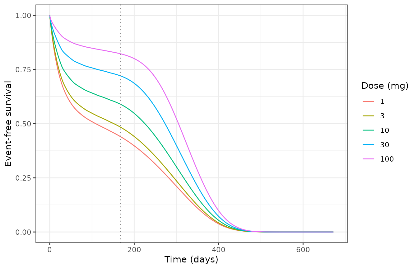
Typical-value event-free survival by dose group. Treatment runs to day 140 (last dose); follow-up continues to day 672, where the rising arm of the bathtub baseline hazard dominates and the curves reconverge.
Virtual cohort
A 200-subject cohort (40 per dose arm) with the paper’s
inter-individual variability on Ke and V2 and
standard-normal draws for both simulation covariates.
rxode2::rxSetSeed(20260902)
set.seed(20260902)

n_per_arm <- 40L
cohort <- tibble::tibble(
  id = seq_len(n_per_arm * length(dose_levels)),
  arm = rep(dose_levels, each = n_per_arm),
  SIMCOV_TI = stats::rnorm(n_per_arm * length(dose_levels)),
  SIMCOV_TV = stats::rnorm(n_per_arm * length(dose_levels))
)

ev_cohort <- lapply(seq_len(nrow(cohort)), function(i) {
  rxode2::et(amt = cohort$arm[[i]], cmt = "depot", time = dose_times) %>%
    rxode2::et(seq(0, 672, by = 7), cmt = "central") %>%
    as.data.frame() %>%
    mutate(id = cohort$id[[i]])
}) %>%
  bind_rows() %>%
  left_join(select(cohort, id, arm, SIMCOV_TI, SIMCOV_TV), by = "id")

s_cohort <- rxode2::rxSolve(mod$simulationModel, events = ev_cohort,
                            omega = mod$omega, returnType = "data.frame",
                            addDosing = FALSE) %>%
  mutate(id = as.integer(as.character(id))) %>%
  left_join(select(cohort, id, arm), by = "id")

# Guard the OTHER direction of the omega leak: IIV must actually have varied.
stopifnot(n_distinct(round(s_cohort$vc, 8)) > 1L,
          n_distinct(round(s_cohort$kel, 8)) > 1L)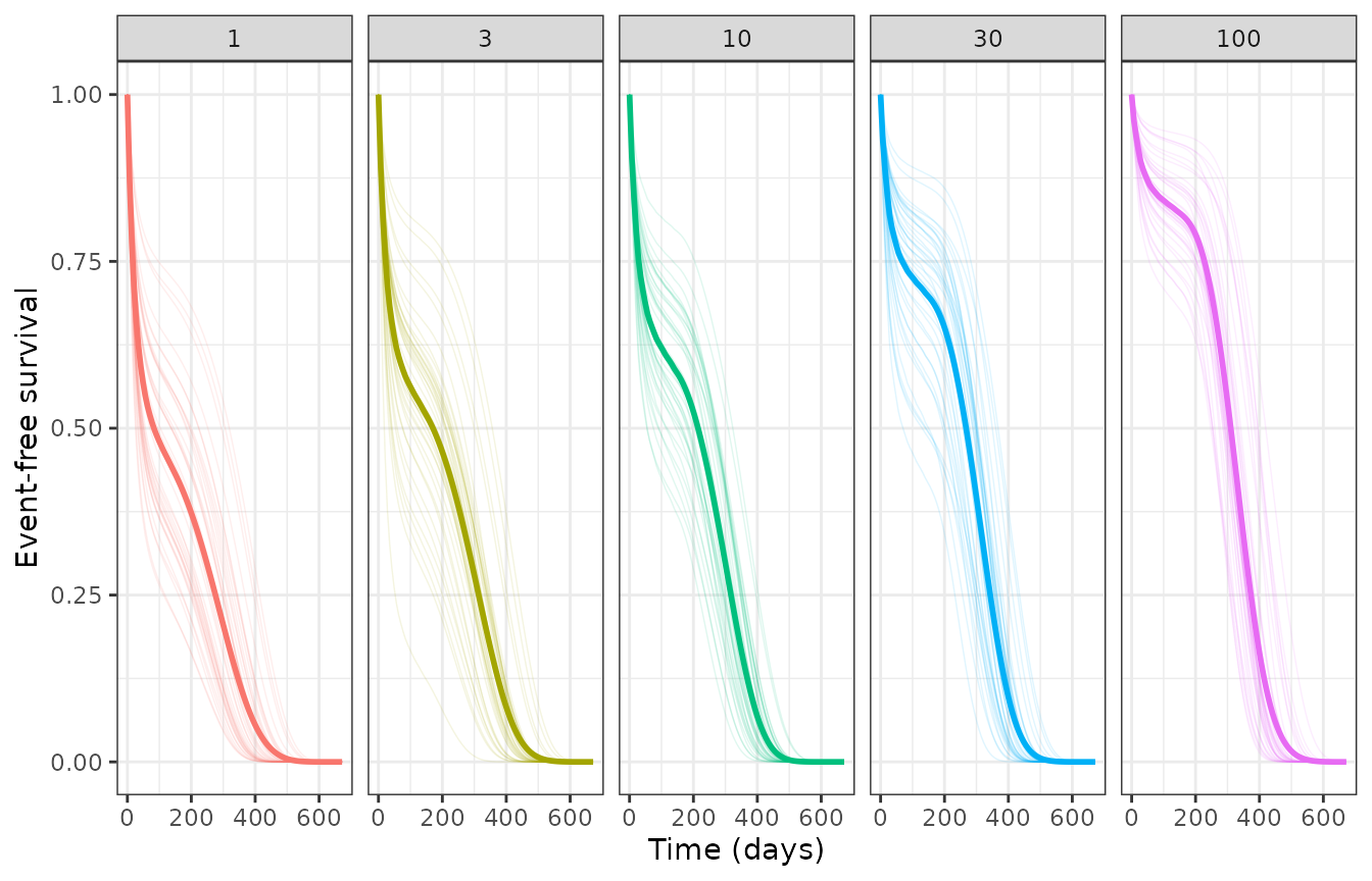
Model-predicted event-free survival across the 200-subject virtual cohort: per-subject curves (thin) with the arm mean (thick). The spread within an arm is driven by the Ke / V2 variability and by the two simulation covariates.
Mean event-free survival at the two on-study landmarks, by arm. The assertion below is deliberately weak: this is a random cohort, so per the repository’s standing guidance only a robust, central comparison between the extreme arms is asserted – not an extreme, and not a per-subject bound. Every strict check on this model lives in the deterministic sections above.
cohort_lm <- s_cohort %>%
  filter(time %in% c(168, 336)) %>%
  group_by(arm, time) %>%
  summarise(mean_sur = mean(sur), .groups = "drop") %>%
  pivot_wider(names_from = time, values_from = mean_sur,
              names_prefix = "Mean S(") %>%
  rename_with(~ paste0(.x, " d)"), starts_with("Mean S(")) %>%
  arrange(arm) %>%
  rename("Dose (mg)" = arm)
knitr::kable(cohort_lm, digits = 4)| Dose (mg) | Mean S(168 d) | Mean S(336 d) |
|---|---|---|
| 1 | 0.4130 | 0.1420 |
| 3 | 0.5039 | 0.1995 |
| 10 | 0.5772 | 0.2221 |
| 30 | 0.6783 | 0.2607 |
| 100 | 0.8110 | 0.4094 |
What this model is not
It is not a fit of anything. Tables 1 and 2 of Lin 2026 report estimates recovered from simulated data by four different methods, together with the printed “true parameter values” the simulation used. It is those true values – the data-generating constants – that are encoded here. The estimates are properties of the estimators being compared, not of a drug, and are not part of this model file.
The semi-parametric Cox stream (Data S1) is likewise not encoded: by design it has no baseline hazard, which is exactly the point of the method, and a model without a baseline hazard cannot be simulated forward.