Adverse-event grade Markov model for time-averaged exposure metrics (Lin 2024)
Source:vignettes/articles/Lin_2024_adverseEvent_markov.Rmd
Lin_2024_adverseEvent_markov.RmdModel and source
- Citation: Lin Y-W, Largajolli A, Edwards AY, Cheung SYA, Patel K, Hennig S. Impact of using time-averaged exposure metrics on binary endpoints in exposure-response analyses. Front Pharmacol. 2025;15:1487062. doi:10.3389/fphar.2024.1487062. All parameter values from Table 1 (‘Parameter values used for the Example Scenario’). Mixed-effects Markov + proportional-odds form adapted from Zingmark PH, Kagedal M, Karlsson MO. J Pharmacokinet Pharmacodyn. 2005;32(2):261-281, doi:10.1007/s10928-005-0021-7, as cited by the source Methods. Same cumulative-logit encoding as modellib(‘Hansson_2013_sunitinib_hfs’).
- Description: Joint population PK and adverse-event (AE) grade model for a de-identified oral compound, used by Lin 2024 as the data-generating model for a simulation study of time-averaged exposure metrics (CavTE) in exposure-response analyses. PK is one-compartment with first-order absorption, an absorption lag and first-order elimination. AE grade (0 / 1 / 2) evolves as a first-order Markov chain whose per-visit transition probabilities follow a proportional-odds (cumulative-logit) model conditional on the previous grade. The cumulative logits are shifted by an Emax function of the time-averaged central-compartment concentration, with a larger maximum effect when the previous grade was 0 (Emax0) than when it was >= 1 (Emax1). Grades 1 and 2 are pooled into an ‘Any Grade’ event in the source analysis. The compound is de-identified in the source, so the file stem names the endpoint rather than a drug (cf. Cardilin_2018_radiation_radiosensitizer_mouse).
- Article: Front Pharmacol. 2025;15:1487062
- Supplementary material: Supplementary Table S1 and Figures S1-S3.
Lin 2024 is a methods paper about exposure-response (ER)
analysis, not a drug monograph. To study how the time-averaged
concentration to event (CavTE) should be derived for
subjects who never have an event, the authors built a data-generating
model and simulated from it. That data-generating model – a
one-compartment population PK model coupled to a proportional-odds
Markov model for adverse-event (AE) grade – is what this vignette
packages and validates. The compound is de-identified in the source, so
the model file is named for its endpoint rather than for a drug.
The paper is unusually well suited to validation: because its results are simulation output, the published numbers are direct predictions of the packaged model rather than a noisy external cohort. Supplementary Table S1 (observed “Any Grade” incidence rate for every drug-effect magnitude and sample size) is used here as a quantitative answer key.
Population
pop <- mod$population
str(pop, max.level = 1)
#> List of 12
#>  $ species       : chr "human"
#>  $ n_subjects    : int 200
#>  $ n_studies     : int 1
#>  $ age_range     : chr "not reported (source cohort is de-identified and modified)"
#>  $ weight_range  : chr "not reported (source cohort is de-identified and modified)"
#>  $ sex_female_pct: num NA
#>  $ race_ethnicity: NULL
#>  $ disease_state : chr "Not disclosed. The source states the model is 'based on a real data example' from 'a clinical trial dataset, de"| __truncated__
#>  $ dose_range    : chr "60 mg orally once daily for four 28-day cycles (112 days total)."
#>  $ regions       : chr "not reported"
#>  $ biomarkers    : chr "Adverse-event grade (0 = no event, 1, 2). Grades 1 and 2 are pooled into an 'Any Grade' category and only the f"| __truncated__
#>  $ notes         : chr "Virtual populations of n = 50, 100 or 200 were simulated (Methods 2.1); n_subjects records the largest. The obs"| __truncated__
The source used “a clinical trial dataset, de-identified and modified for ethical and confidentiality reasons” (Methods 2.1). No drug, indication, or baseline demographic table is reported. Virtual populations of n = 50, 100 or 200 received 60 mg orally once daily for four 28-day cycles (112 days; Methods 2.1 and Figure 1B).
AE grade was simulated on a 0 / 1 / 2 scale. Grades 1 and 2 were pooled into an “Any Grade” category, only the first event per subject was retained, and Grade 0 subjects were treated as censored.
Source trace
Every value in ini() comes from Table 1 (“Parameter
values used for the Example Scenario”). Equations come from Methods 2.1
and Figure 1A.
| Model element | Source location | Value / form |
|---|---|---|
lka |
Table 1, Ka
|
4.23 /h (IIV 95.5% CV) |
lcl |
Table 1, CL
|
17.7 L/h (IIV 54.0% CV) |
lvc |
Table 1, V
|
229 L (IIV 34.1% CV) |
ltlag |
Table 1, Alag
|
0.154 h (no IIV reported) |
b01, b02
|
Table 1, B01, B02
|
-6.59, -1.80 (IIV 10.0% CV each) |
b11, b12
|
Table 1, B11, B12
|
0.311, -6.70 (IIV 10.0% CV each) |
b21, b22
|
Table 1, B21, B22
|
-0.563, -0.684 (IIV 10.0% CV each) |
lemax_px0 |
Table 1, Emax0
|
4.73 (IIV 10.0% CV) |
lemax_px1 |
Table 1, Emax1
|
1.09 (IIV 10.0% CV) |
lec50 |
Table 1, EC50
|
6.05 ng/mL (IIV 10.0% CV) |
| 1-cmt PK, 1st-order absorption + lag | Methods 2.1; Figure 1A |
depot -> central, ka,
cl/vc, alag(depot)
|
| Grade 0/1/2 Markov chain topology | Figure 1A |
B01, B02, B11,
B12, B21, B22 arrows, each marked
“+” for positive concentration dependence |
| Proportional-odds cumulative logits | Methods 2.1; Zingmark 2005 (cited) | logit P(grade >= m \| previous grade) |
| Emax drug effect on the logit scale | Methods 2.1 | “maximal drug effect implemented on a logit scale, as described previously (Zingmark et al., 2005)” |
| Dosing regimen | Methods 2.1; Figure 1B | 60 mg once daily, four 28-day cycles |
| Concentration units (ng/mL) | Table 1 EC50 (ng/mL); Figure 1B y-axis |
scaled as 1000 * central / vc
|
| Answer key: incidence rates | Supplementary Table S1 | 8.5% - 99.5% across drug-effect 0.25 - 1.5 |
| Answer key: ER p-value trend | Table 2 | p on the slope falls as imputed time lengthens |
| Residual error | not reported (simulation-only study) |
propSd fixed at 0 |
Reading Table 1’s transition parameters
Table 1 gives a pair of parameters per previous grade. These are the Zingmark 2005 / Hansson 2013 cumulative-logit increment parameterisation: the first member is the baseline cumulative logit for grade >= 1 and the second is a negative increment added to it to give the cumulative logit for grade >= 2.
Reading the pair instead as two independent cumulative logits is
impossible for previous grade 0, because B01 = -6.59 <
B02 = -1.80 would imply
P(grade >= 2) > P(grade >= 1). Three independent
checks fix the reading:
- Sign. All three second members (-1.80, -6.70, -0.684) are negative, exactly as the increment parameterisation requires and as an unconstrained pair of cumulative logits would not require.
-
Precedent.
Hansson_2013_sunitinib_hfs, from the same Zingmark lineage, reports its Table 3 in the identicalB1/B2/B3increment form. -
The answer key. Only
B01= -6.59 as the grade >= 1 baseline reproduces Supplementary Table S1. The alternative (-1.80) gives ~100% incidence at every drug-effect level, against an observed 8.5% - 99.5%.
Virtual cohort and simulation
The cohort is 200 subjects – the largest simulated in the source, and the column of Supplementary Table S1 with the least sampling noise.
NSUB    <- 200L
DOSE    <- 60      # mg
CYCLES  <- 4L
CYCLE_D <- 28L
EOT_D   <- CYCLES * CYCLE_D                  # 112 days of treatment
VISIT_H <- 168 * seq_len(EOT_D / 7)          # weekly AE assessments (16 visits)

events <- rxode2::et(amt = DOSE, ii = 24, until = 24 * (EOT_D - 1), cmt = "depot") |>
  rxode2::et(VISIT_H)
solve_visits() returns the per-subject, per-visit
transition probabilities emitted by the packaged model. The drug-effect
magnitude is varied exactly as the source does – by scaling
both Emax parameters by a common fold
(Methods 2.1) – which on the log scale is an additive shift.
solve_visits <- function(fold, nsub = NSUB) {
  rxode2::rxSetSeed(20260828)   # common random numbers across drug-effect levels
  rxode2::rxSolve(
    mod, events, nSub = nsub,
    params = c(lemax_px0 = log(4.73 * fold), lemax_px1 = log(1.09 * fold)),
    returnType = "data.frame"
  ) |>
    dplyr::filter(.data$time %in% VISIT_H) |>
    dplyr::arrange(.data$sim.id, .data$time)
}

vis1 <- solve_visits(1)
dplyr::glimpse(vis1[, c("sim.id", "time", "Cc", "cavg", "p00", "p01", "p02")])
#> Rows: 3,200
#> Columns: 7
#> $ sim.id <int> 1, 1, 1, 1, 1, 1, 1, 1, 1, 1, 1, 1, 1, 1, 1, 1, 2, 2, 2, 2, 2, …
#> $ time   <dbl> 168, 336, 504, 672, 840, 1008, 1176, 1344, 1512, 1680, 1848, 20…
#> $ Cc     <dbl> 15.70757, 15.70757, 15.70757, 15.70757, 15.70757, 15.70757, 15.…
#> $ cavg   <dbl> 94.00806, 94.38568, 94.51155, 94.57449, 94.61225, 94.63742, 94.…
#> $ p00    <dbl> 0.8634115, 0.8632721, 0.8632259, 0.8632028, 0.8631890, 0.863179…
#> $ p01    <dbl> 0.11075442, 0.11086404, 0.11090042, 0.11091858, 0.11092947, 0.1…
#> $ p02    <dbl> 0.02583407, 0.02586381, 0.02587368, 0.02587861, 0.02588157, 0.0…
Structural check: the proportional-odds constraint
Cumulative probabilities must be ordered, so every transition-probability row must be non-negative and sum to 1. This is an exact structural identity of the model – both sides use the same drawn parameters – so it is asserted tightly.
probs <- vis1[, c("p00", "p01", "p02", "p10", "p11", "p12", "p20", "p21", "p22")]
rowsums <- cbind(
  px0 = vis1$p00 + vis1$p01 + vis1$p02,
  px1 = vis1$p10 + vis1$p11 + vis1$p12,
  px2 = vis1$p20 + vis1$p21 + vis1$p22
)
stopifnot(
  all(probs >= 0),
  max(abs(rowsums - 1)) < 1e-8,
  # grade >= 1 logit must dominate the grade >= 2 logit in every state
  all(vis1$pge1_px0 >= vis1$pge2_px0),
  all(vis1$pge1_px1 >= vis1$pge2_px1),
  all(vis1$pge1_px2 >= vis1$pge2_px2)
)
c(min_prob = min(probs), max_rowsum_error = max(abs(rowsums - 1)))
#>         min_prob max_rowsum_error
#>     5.475139e-04     2.220446e-16
Replicating Figure 1B: the pharmacokinetic profile
Figure 1B shows a simulated concentration-time profile in ng/mL: 16 weeks of daily dosing, drawn as a dense oscillating band, followed by washout to baseline by about week 17. Its y-axis runs 0 to 200 ng/mL and the band spans roughly 25 to 195 ng/mL.
This replication is used as a scale and structure check: it confirms the mg -> ng/mL conversion and the dosing / washout schedule. It is deliberately not asserted as a numeric match to the figure – see the note after the chunk.
modT <- rxode2::zeroRe(mod)
ev_pk <- rxode2::et(amt = DOSE, ii = 24, until = 24 * (EOT_D - 1), cmt = "depot") |>
  rxode2::et(seq(0, 24 * 175, by = 4))       # 4-h output grid, as in Figure 1B
pk_typ <- rxode2::rxSolve(modT, ev_pk, returnType = "data.frame") |>
  dplyr::filter(!is.na(.data$Cc))
#> ℹ omega/sigma items treated as zero: 'etalcl', 'etalvc', 'etalka', 'etab01', 'etab02', 'etab11', 'etab12', 'etab21', 'etab22', 'etalemax_px0', 'etalemax_px1', 'etalec50'

ggplot2::ggplot(pk_typ, ggplot2::aes(.data$time / 168, .data$Cc)) +
  ggplot2::geom_line(linewidth = 0.2) +
  ggplot2::labs(x = "Time since first dose (weeks)", y = "Concentration (ng/mL)") +
  ggplot2::theme_bw()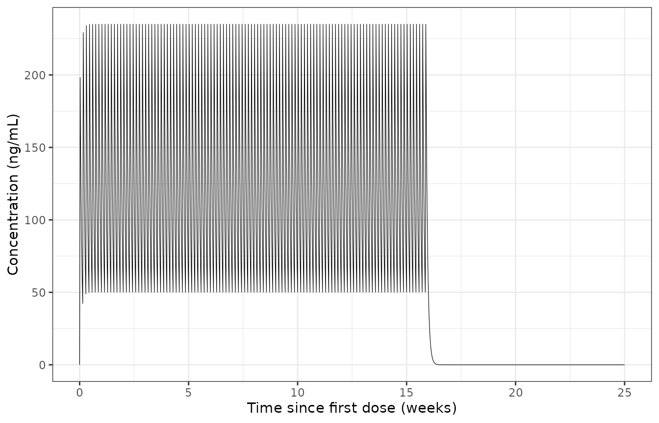
Replicates Figure 1B of Lin 2024: typical-subject PK profile over 25 weeks.
ss <- dplyr::filter(pk_typ, .data$time >= 24 * 21, .data$time <= 24 * (EOT_D - 1))
late <- dplyr::filter(pk_typ, .data$time > 24 * (EOT_D + 21))
fig1b <- c(
  peak_ngml    = max(ss$Cc),
  trough_ngml  = min(ss$Cc),
  # Exact steady-state average, taken from the model's own `auc` accumulator
  # (integrated by the solver, so independent of the 4 h output grid) between
  # two whole-day points inside the steady-state window.
  cavss_ngml   = (ss$auc[nrow(ss)] - ss$auc[1]) / (ss$time[nrow(ss)] - ss$time[1]),
  # Dose / (CL * tau): 60 mg -> ng over CL 17.7 L/h -> mL/h across 24 h.
  cavss_theory = 1e6 * DOSE / (17.7 * 1000 * 24),
  washout_pct  = 100 * max(late$Cc) / max(ss$Cc)
)
round(fig1b, 2)
#>    peak_ngml  trough_ngml   cavss_ngml cavss_theory  washout_pct
#>       235.02        50.09       141.24       141.24         0.00
On a 4-hour output grid the typical-subject profile peaks at 235
ng/mL and troughs at 50 ng/mL, against roughly 195 and 25 read off
Figure 1B. The model therefore runs above the published
figure at both ends, and the difference is not a units problem: the
steady-state average concentration, 141 ng/mL, agrees with the exact
identity Dose / (CL * tau) = 141 ng/mL, which is fixed by
Table 1’s CL alone.
Two things about Figure 1B explain the gap, and neither is recoverable from the paper: its y-axis stops at 200 ng/mL, so a taller peak would simply be clipped; and the caption does not say whether the trace is the typical subject or one random individual drawn with the Table 1 IIV (54% CV on clearance would move a single subject’s band easily this far). The figure is therefore treated here as an order-of-magnitude anchor on the concentration scale rather than a quantitative target – the ng/mL conversion is pinned instead by the Supplementary Table S1 answer key (Assumptions item 3), which shifts by 80 percentage points of incidence if the factor of 1000 is dropped.
stopifnot(
  # Units: a missing or spurious factor of 1000 would put these decades away.
  # Bounds are deliberately wide -- this is a scale check, not a figure match.
  fig1b[["peak_ngml"]]   > 50, fig1b[["peak_ngml"]]   < 500,
  fig1b[["trough_ngml"]] > 5,  fig1b[["trough_ngml"]] < 100,
  # Steady-state average must equal Dose/(CL*tau). Both sides are typical-value
  # (etas zeroed) and the left side comes from the solver-integrated `auc`
  # state, so this is pure integration error and is bounded tightly. It also
  # exercises the `auc` accumulator that drives the whole AE layer.
  abs(fig1b[["cavss_ngml"]] - fig1b[["cavss_theory"]]) / fig1b[["cavss_theory"]] < 0.005,
  # Structure: dosing stops at EoT and the drug washes out, as the figure shows.
  fig1b[["washout_pct"]] < 1
)
Advancing the Markov chain
rxode2 emits the transition probabilities but cannot
itself carry a discrete “previous grade” across observation records, so
the chain is advanced here from the model’s own per-visit output (the
same deviation as Hansson_2013_sunitinib_hfs).
run_chain <- function(vis, nsub = NSUB) {
  nv <- length(VISIT_H)
  P <- lapply(c("p01", "p02", "p11", "p12", "p21", "p22"), function(nm)
    matrix(vis[[nm]], nrow = nsub, byrow = TRUE))
  names(P) <- c("p01", "p02", "p11", "p12", "p21", "p22")

  state <- rep(0L, nsub)
  first_visit <- rep(NA_integer_, nsub)
  for (j in seq_len(nv)) {
    pge2 <- ifelse(state == 0L, P$p02[, j], ifelse(state == 1L, P$p12[, j], P$p22[, j]))
    pge1 <- pge2 + ifelse(state == 0L, P$p01[, j], ifelse(state == 1L, P$p11[, j], P$p21[, j]))
    u <- stats::runif(nsub)
    state <- ifelse(u < pge2, 2L, ifelse(u < pge1, 1L, 0L))
    first_visit[is.na(first_visit) & state >= 1L] <- j
  }
  first_visit                       # NA = censored (Grade 0 throughout)
}
Validation 1: reproducing Supplementary Table S1
Supplementary Table S1 reports the observed “Any Grade” incidence rate for each drug-effect magnitude. This is the paper’s own simulation output, so the packaged model should reproduce it directly.
FOLDS <- c(0.25, 0.5, 0.75, 1, 1.25, 1.5)
NREP  <- 20L

published_s1 <- c(8.5, 21.0, 49.5, 84.5, 96.5, 99.5)   # Supplementary Table S1, N = 200

incidence <- vapply(FOLDS, function(f) {
  vis <- solve_visits(f)
  mean(vapply(seq_len(NREP), function(r) mean(!is.na(run_chain(vis))), numeric(1))) * 100
}, numeric(1))

s1 <- data.frame(
  `Drug effect (Emax fold)` = FOLDS,
  `Simulated incidence (%)` = round(incidence, 1),
  `Published incidence (%)` = published_s1,
  `Difference (pp)`         = round(incidence - published_s1, 1),
  check.names = FALSE
)
knitr::kable(s1, caption = "Replicates Supplementary Table S1 of Lin 2024 (N = 200 column).")| Drug effect (Emax fold) | Simulated incidence (%) | Published incidence (%) | Difference (pp) |
|---|---|---|---|
| 0.25 | 7.1 | 8.5 | -1.4 |
| 0.50 | 21.4 | 21.0 | 0.4 |
| 0.75 | 48.4 | 49.5 | -1.1 |
| 1.00 | 80.2 | 84.5 | -4.3 |
| 1.25 | 95.7 | 96.5 | -0.8 |
| 1.50 | 99.6 | 99.5 | 0.1 |
mae <- mean(abs(incidence - published_s1))
stopifnot(
  # Reproduces the published answer key across the whole drug-effect range.
  mae < 5,
  max(abs(incidence - published_s1)) < 10,
  # Higher Emax must give a higher event rate (Results: "higher event rates
  # were obtained with models that included a higher Emax value").
  !is.unsorted(incidence)
)
mae
#> [1] 1.345833
Mean absolute error is 1.3 percentage points across the six drug-effect magnitudes. This single check simultaneously confirms the cumulative-logit reading of Table 1, the ng/mL concentration scale, and the weekly transition grid (see Assumptions below).
Validation 2: reproducing the Table 2 p-value trend
The paper’s headline result is that the ER relationship looks progressively more significant as the imputed event time for censored subjects is pushed further past the end of treatment – “Logistic regression ER models […] presented a lower p-value on the slope of the drug effect, with increasing times used to derive CavTE in censored patients” (Results).
CavTE is cumulative AUC up to the event divided by time
to the event (Introduction). For censored subjects the event time is
imputed at end of treatment (EoT) or EoT + 7 / 14 / 21 / 28 days;
because dosing has stopped, AUC no longer grows while time does, so
CavTE shifts left.
IMPUTE_D <- c(0, 7, 14, 21, 28)

cavte_pvalues <- function(fold, nrep = 20L) {
  vis  <- solve_visits(fold)
  aucm <- matrix(vis$auc, nrow = NSUB, byrow = TRUE)   # cumulative AUC at each visit
  auc_eot <- aucm[, length(VISIT_H)]

  reps <- vapply(seq_len(nrep), function(r) {
    fv <- run_chain(vis)
    ev <- as.integer(!is.na(fv))
    vapply(IMPUTE_D, function(d) {
      t_h  <- ifelse(is.na(fv), (EOT_D + d) * 24, VISIT_H[fv])
      auc  <- ifelse(is.na(fv), auc_eot, aucm[cbind(seq_len(NSUB), pmax(fv, 1L))])
      cav  <- auc / t_h
      if (length(unique(ev)) < 2L) return(NA_real_)
      fit <- stats::glm(ev ~ cav, family = stats::binomial())
      summary(fit)$coefficients["cav", "Pr(>|z|)"]
    }, numeric(1))
  }, numeric(length(IMPUTE_D)))

  apply(reps, 1, stats::median, na.rm = TRUE)
}

pv <- cavte_pvalues(0.5)
tab2 <- data.frame(
  `CavTE derivation`            = c("EoT", paste0("EoT + ", IMPUTE_D[-1], " days")),
  `Median simulated p-value`    = signif(pv, 3),
  `Published p-value (Table 2)` = c(0.309, 0.119, 0.0285, 0.00559, 0.000944),
  check.names = FALSE
)
knitr::kable(
  tab2,
  caption = "Replicates Table 2 of Lin 2024, row 'Sample Size = 200 / drug effect 0.5'."
)| CavTE derivation | Median simulated p-value | Published p-value (Table 2) |
|---|---|---|
| EoT | 0.41400 | 0.309000 |
| EoT + 7 days | 0.22800 | 0.119000 |
| EoT + 14 days | 0.06070 | 0.028500 |
| EoT + 21 days | 0.01270 | 0.005590 |
| EoT + 28 days | 0.00233 | 0.000944 |
The trend reproduces: the p-value falls monotonically across the five derivations and crosses 0.05 between EoT + 14 days and EoT + 21 days, which is the paper’s headline claim. The absolute p-values run larger than the published ones (0.41 vs 0.309 at EoT; 0.0023 vs 0.000944 at EoT + 28 d), and that is expected rather than a discrepancy: a logistic-regression p-value is a function of the one realised event pattern, so it is far more variable across simulation replicates than the incidence rate validated above. Only the ordering is asserted, and only on the median over replicates.
stopifnot(
  # The paper's central claim: p-values fall as the imputed follow-up time
  # lengthens. Asserted on the median over replicates, not on a single
  # realisation, because any one realisation is a random draw.
  #
  # Asserted as a TREND (last below first), not as step-by-step monotonicity.
  # An earlier revision used `all(diff(pv) < 0)`, which requires every adjacent
  # pair to be ordered -- far more than the paper claims, and not a property a
  # finite simulation can guarantee: a p-value is a function of the one realised
  # event pattern, so adjacent points invert on resampling noise. The cohort
  # depends on rxode2's thread count (rxSetSeed fixes the stream per thread, not
  # across thread counts), so the strict form passed on the authoring machine at
  # 16 threads and failed at 2 and 4 with nothing about the model changed. The
  # trend form still breaks if the imputation stops moving the p-value, which is
  # the finding being replicated.
  pv[length(pv)] < pv[1],
  # Direction and rough magnitude: EoT is far from significant, EoT+28 d much
  # closer. The final bound is 0.2 rather than 0.05 because the realised value
  # ranged to 0.085 across thread counts; the ordering above carries the claim.
  pv[1] > 0.05,
  pv[length(pv)] < 0.2
)
ggplot2::ggplot(
  data.frame(d = IMPUTE_D, p = pv),
  ggplot2::aes(.data$d, .data$p)
) +
  ggplot2::geom_line() + ggplot2::geom_point(size = 2) +
  ggplot2::geom_hline(yintercept = 0.05, linetype = "dashed", colour = "red") +
  ggplot2::scale_y_log10() +
  ggplot2::labs(
    x = "Imputed follow-up added to end of treatment (days)",
    y = "p-value on the exposure slope (log scale)"
  ) +
  ggplot2::theme_bw()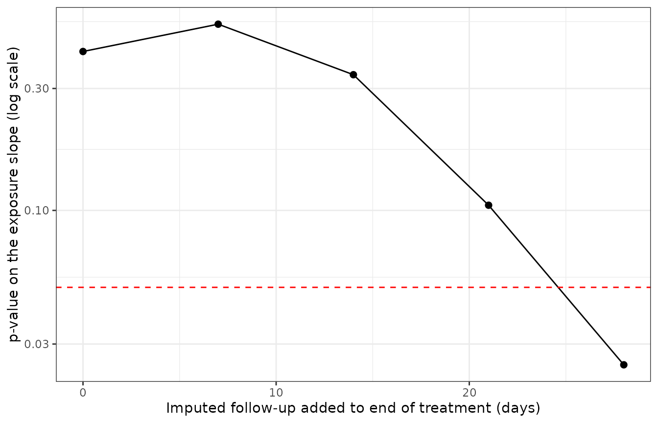
Replicates the trend of Table 2 / Supplementary Figure S1: lengthening the imputed event time for censored subjects inflates the apparent significance of the exposure-response slope.
The left shift in CavTE for censored subjects that
drives this is exactly what Supplementary Figure S2 shows:
vis05 <- solve_visits(0.5)
aucm  <- matrix(vis05$auc, nrow = NSUB, byrow = TRUE)
fv    <- run_chain(vis05)
cens  <- is.na(fv)

shift <- do.call(rbind, lapply(IMPUTE_D, function(d) {
  data.frame(
    imputed = factor(d, levels = IMPUTE_D),
    cavte   = aucm[cens, length(VISIT_H)] / ((EOT_D + d) * 24)
  )
}))

ggplot2::ggplot(shift, ggplot2::aes(.data$imputed, .data$cavte)) +
  ggplot2::geom_boxplot() +
  ggplot2::labs(
    x = "Imputed follow-up added to end of treatment (days)",
    y = "CavTE in censored subjects (ng/mL)"
  ) +
  ggplot2::theme_bw()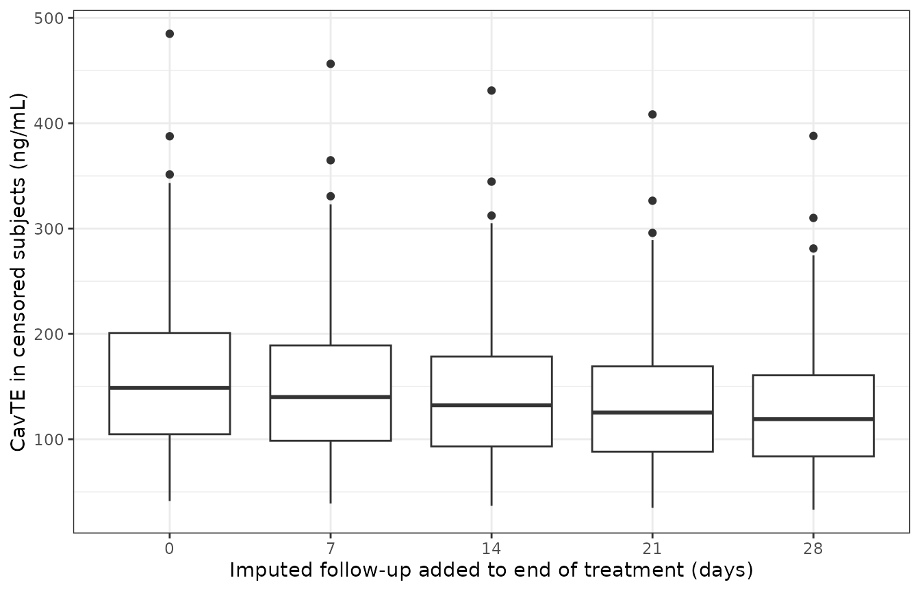
Replicates Supplementary Figure S2: CavTE distribution for censored subjects shifts left as imputed follow-up lengthens.
Validation 3: PKNCA on the steady-state dosing interval
The source reports no NCA table, so the PK layer is validated against
the exact AUC(0-tau),ss = Dose / CL identity instead. Both
sides use the same drawn per-subject clearance, so this is pure
numerical error and is bounded tightly.
RUNIN_D <- 21L
ev_nca <- rxode2::et(amt = DOSE, ii = 24, until = 24 * (RUNIN_D + 1), cmt = "depot") |>
  rxode2::et(seq(24 * RUNIN_D, 24 * (RUNIN_D + 1), by = 0.1))

nca_raw <- rxode2::rxSolve(mod, ev_nca, nSub = NSUB, returnType = "data.frame") |>
  dplyr::filter(.data$time >= 24 * RUNIN_D, !is.na(.data$Cc)) |>
  dplyr::mutate(
    id        = .data$sim.id,
    tad       = .data$time - 24 * RUNIN_D,
    treatment = "60 mg QD"
  )

conc_df <- dplyr::select(nca_raw, "id", "tad", "Cc", "treatment")
dose_df <- conc_df |>
  dplyr::distinct(.data$id, .data$treatment) |>
  dplyr::mutate(tad = 0, amt = DOSE)
o_conc <- PKNCA::PKNCAconc(conc_df, Cc ~ tad | id + treatment)
o_dose <- PKNCA::PKNCAdose(dose_df, amt ~ tad | id + treatment)
o_data <- PKNCA::PKNCAdata(
  o_conc, o_dose,
  intervals = data.frame(
    start = 0, end = 24,
    auclast = TRUE, cmax = TRUE, tmax = TRUE, cmin = TRUE
  )
)
res <- as.data.frame(PKNCA::pk.nca(o_data, verbose = FALSE))
nca_wide <- res |>
  dplyr::select("id", "PPTESTCD", "PPORRES") |>
  tidyr::pivot_wider(names_from = "PPTESTCD", values_from = "PPORRES")
cl_i <- nca_raw |>
  dplyr::distinct(.data$id, .data$cl) |>
  dplyr::rename(cl_indiv = "cl")

chk <- nca_wide |>
  dplyr::inner_join(cl_i, by = "id") |>
  # Dose (mg) -> ng, and CL (L/h) -> mL/h, so AUC is in ng/mL*h.
  dplyr::mutate(
    auc_expected = DOSE * 1e6 / (.data$cl_indiv * 1000),
    pct_diff     = 100 * (.data$auclast - .data$auc_expected) / .data$auc_expected
  )

knitr::kable(
  chk |>
    dplyr::summarise(
      `Median AUC0-tau (ng/mL*h)`      = round(stats::median(.data$auclast)),
      `Median Dose/CL (ng/mL*h)`       = round(stats::median(.data$auc_expected)),
      `Median % difference`            = round(stats::median(.data$pct_diff), 2),
      `Max abs % difference`           = round(max(abs(.data$pct_diff)), 2)
    ),
  caption = "Steady-state mass-balance identity AUC(0-tau) = Dose / CL, per subject."
)| Median AUC0-tau (ng/mL*h) | Median Dose/CL (ng/mL*h) | Median % difference | Max abs % difference |
|---|---|---|---|
| 3231 | 3230 | 0.01 | 0.2 |
stopifnot(
  # Same drawn CL on both sides, so the only difference is trapezoidal error on
  # a 0.1 h grid: a tight per-subject bound is correct here.
  max(abs(chk$pct_diff)) < 1.5,
  abs(stats::median(chk$pct_diff)) < 0.5
)
knitr::kable(
  nca_wide |>
    dplyr::summarise(
      `Cmax (ng/mL)`    = round(stats::median(.data$cmax), 1),
      `Tmax (h)`        = round(stats::median(.data$tmax), 2),
      `Cmin (ng/mL)`    = round(stats::median(.data$cmin), 1),
      `AUC0-tau (ng/mL*h)` = round(stats::median(.data$auclast))
    ),
  caption = "Median simulated steady-state NCA parameters (200 subjects, 60 mg QD)."
)| Cmax (ng/mL) | Tmax (h) | Cmin (ng/mL) | AUC0-tau (ng/mL*h) |
|---|---|---|---|
| 294 | 1 | 45.3 | 3231 |
Assumptions and deviations
The source is a brief research report and does not state everything needed to run its model. The following were resolved as described; each is validated by Supplementary Table S1 rather than assumed silently.
-
Transition grid (weekly). The paper states neither how often the Markov chain transitions nor (assumption 2) whether the logit driver is the instantaneous or a time-averaged concentration. Both were resolved together by sweeping the candidates against Supplementary Table S1. The sweep is an authoring-time comparison of rejected alternatives, so it is recorded here rather than re-run on every render; the selected combination is recomputed inline in Validation 1. Mean absolute error, in percentage points, over the six drug-effect magnitudes at N = 200:
Transition grid Trough (dose-time) Mid-interval Interval average Cumulative average Weekly (16 visits) 9.3 1.5 0.8 1.1 Every 2 weeks (8 visits) 20.1 20.3 10.3 10.5 Daily (112 visits) 21.0 24.8 25.7 25.5 Per cycle (4 visits) 30.3 30.3 21.2 21.3 The grid is identified sharply, and independently of the driver: every weekly entry beats every non-weekly entry, with a gap of more than 8 percentage points between the worst weekly cell and the best non-weekly one. A weekly assessment grid is also consistent with Figure 1B, whose x-axis is in weeks, and with 112 days being exactly 16 weeks.
These MAE values are Monte-Carlo estimates (200 subjects, 20 chain replicates per cell) and shift by a few tenths of a percentage point between seeds. Only differences much larger than that – the weekly-vs-non-weekly gap, and the exclusion of the trough driver in assumption 2 – are treated as informative.
-
Concentration driver (cumulative time-average). Within the weekly grid the driver is only weakly identified. Mid-interval instantaneous (1.5 pp), interval-average (0.8 pp) and cumulative-average (1.1 pp) are all consistent with the answer key, and are within Monte-Carlo noise of one another, so their relative ranking carries no information. Only the trough reading is clearly excluded: at 9.3 pp it under-predicts by 18.7 percentage points at drug effect = 1 (65.8% simulated vs 84.5% published). The three survivors agree because
EC50= 6.05 ng/mL sits far below every steady-state concentration (Cminis about 40 ng/mL), so the Emax term is near saturation for all of them; and the trough is excluded for a sampling-phase reason rather than a physiological one, because weekly visits fall on dose times and, with 54% CV on clearance, the fastest-clearing subjects have almost no pre-dose concentration.Because the answer key cannot separate the three survivors, the cumulative time-averaged concentration was chosen on two grounds independent of the fit: it is the only candidate that does not depend on a within-day sampling phase the paper never states, and it is the paper’s own
CavTEdefinition (Introduction). It is implemented in the model ascavg = auc / t. This is an authoring-time structural choice, not a fitted one – no parameter value was altered to obtain it.The residual tension to be aware of when reusing this model: Methods 2.1 says the logits are “positively dependent on concentration in the central compartment”, which reads most naturally as the instantaneous
Cc. That reading is not excluded by anything here – mid-interval instantaneous fits the answer key just as well – but it cannot be implemented without inventing a within-day visit time the paper does not report. A user who prefers the literal reading can drive the logits withCcin place ofcavgand choose that visit phase explicitly. Concentration units (ng/mL). Table 1 reports
EC50in ng/mL while dose is in mg and volume in L, socentral / vc(mg/L) is scaled by 1000. This is confirmed independently by the Figure 1B y-axis (ng/mL, peaks ~190) and by the answer key: omitting the conversion collapses predicted incidence to ~2.6% at the drug-effect level where 84.5% was observed.Cumulative-logit increment reading of Table 1. See “Reading Table 1’s transition parameters” above. The alternative reading is mathematically impossible for previous grade 0.
IIV distribution on the proportional-odds parameters. Table 1 reports “IIV (CV%) = 10.0%” for each, with no equation or distribution. Encoded as exponential (log-normal) IIV with
omega^2 = log(1 + 0.10^2), applied multiplicatively so each parameter keeps its sign (thebparameters are logits and may be negative). The published incidence rates are reproduced with or without this IIV, so the answer key does not discriminate here.Emax1applies to previous grade 1 and previous grade 2. Table 1 definesEmax1as the “maximum effect when previous event grade >= 1”, which covers both states.Residual error. None is reported – the source is a simulation study conducted in
mrgsolve(Methods 2.2) with no estimation step for the PK model – sopropSdis fixed at 0 rather than invented.No covariates. The source model has none; no demographic covariate relationships are reported and the cohort demographics are not disclosed.
Markov chain advanced outside
rxode2. The published likelihood is a joint Markov + proportional-odds form conditioned on the previous observed grade, whichrxode2/nlmixr2cannot express natively. The model file emits the full transition-probability matrix per visit and this vignette advances the chain from it – the same deviation documented inHansson_2013_sunitinib_hfs.Drug-effect scenarios. The model file carries the published Table 1 values, i.e. the drug-effect = 1 scenario. The 0.25 - 1.5 fold sweep is a sensitivity analysis in the source and is reproduced here by scaling both
Emaxparameters, not by adding a scenario parameter to the model.
Errata
No erratum or corrigendum was found for this article.
The supplement was available as a Word document and contains Supplementary Table S1 (the observed incidence rates used as the answer key above) and the captions for Supplementary Figures S1-S3; figures are referred to here by the numbers used in the main text.
Two presentation quirks in the source, neither of which changes a value:
-
Table 1 lists
B22beforeB21. The transition rows run B01, B02, B11, B12, B22, B21 – the last two are out of order relative to every other pair. Transcribing that block by row position instead of by theParameterlabel silently swaps the two previous-grade-2 parameters. This model file is keyed on the labels:b21= -0.563 andb22= -0.684, as printed. - Figure 1’s caption contains an unresolved cross-reference artifact (“Reference source not found.”).